TESS has produced more than 7,800 planet candidates and fewer than 720 are confirmed. Most of the rest are eclipsing binaries, background blends or instrumental artifacts that happen to look like transits. Checking that backlog by hand does not scale, which is why automated vetting is now a standard step. This post builds a two-branch CNN that separates real planet signals from the usual impostors using phase-folded light curves.
The discriminative counterpart
The previous post was generative: given a transit, infer its parameters. This one is discriminative: given a candidate, decide whether it is a planet at all. The two go together. Vetting triages the pile, SBI characterizes what survives.
A synthetic but honest dataset
I build the training set from three populations, because the interesting question is not whether a CNN can spot a deep clean dip but whether it can resist the things that mimic a planet.
- Planets: limb-darkened transits from
batman, shallow, sometimes grazing. - Eclipsing binaries: a stellar companion modelled with the same transit code, so the eclipse shape is realistic rather than a giveaway sharp V. Depths overlap the planet range at the low end, and a weak secondary eclipse shows up only part of the time.
- Stellar variability: smooth quasi-periodic wiggles with no eclipse.
The overlap is deliberate. A grazing eclipsing binary with no visible secondary looks almost exactly like a small planet, and that is the case real pipelines actually get wrong.
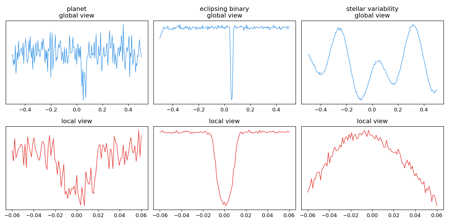
Each candidate is turned into two views, following the Astronet recipe: a low-resolution global view of the full phase-folded curve, and a high-resolution local view zoomed on the transit.
The model
Two small 1D-CNN branches, one per view, concatenated into a dense head.
class VetNet(nn.Module):
    def __init__(self):
        super().__init__()
        self.g = branch(N_GLOBAL)   # global-view conv stack
        self.l = branch(N_LOCAL)    # local-view conv stack
        self.head = nn.Sequential(
            nn.LazyLinear(64), nn.ReLU(), nn.Dropout(0.3), nn.Linear(64, 1))

    def forward(self, g, l):
        return self.head(torch.cat([self.g(g), self.l(l)], 1)).squeeze(1)
Training on 6000 synthetic light curves took a few seconds on a laptop GPU (Apple MPS).
Results
On 2000 held-out candidates:
ROC AUC = 0.9602
average precision = 0.9376
@0.5  precision 0.890  recall 0.983  (TP 978  FP 121  FN 17  TN 884)
@precision>=0.95: recall 0.532
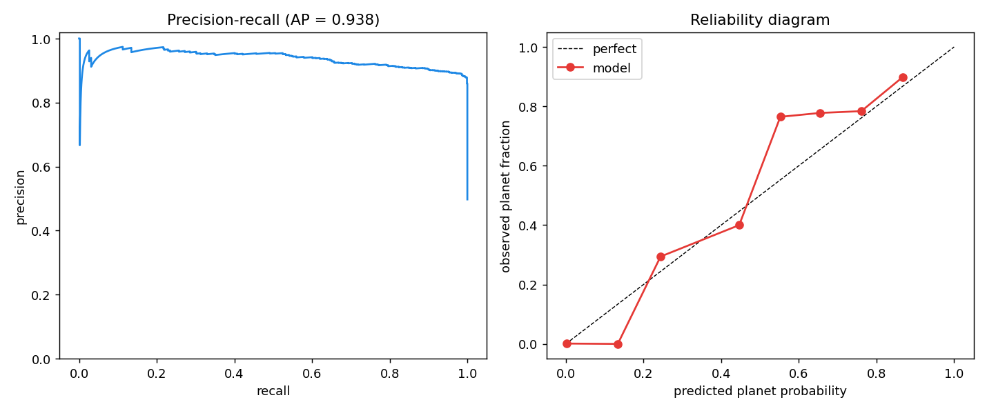
The threshold trade-off is the whole story, and it is why accuracy alone is a useless number here. At the default 0.5 threshold the net catches 98% of planets but only 89% of what it flags is real. Push the purity requirement up to 95% and recall collapses to 53%. You cannot have both, because the grazing binaries genuinely overlap the planets, and no amount of training removes information that the light curve does not contain. The right operating point depends on what the follow-up costs: spectroscopy time is expensive, so a real survey leans toward purity and accepts that it is throwing away half the real planets at that setting.
The reliability diagram says the probabilities are roughly trustworthy, tracking the diagonal with a mild wobble, so you can reason about the threshold instead of treating the output as an opaque score.
Failure cases
The 17 missed planets are the grazing, shallow ones whose V-shaped dip is indistinguishable from an eclipsing binary in a single phase-folded curve. The 121 false positives are the mirror image: shallow binaries with no secondary eclipse in view. Both failures point at the same missing information. A real vetting model adds the features that break the degeneracy, the centroid shift during transit (a blended binary moves on the detector, a planet does not) and the odd-even depth difference (a binary often shows alternating deep and shallow eclipses). Those are extra input heads, not a deeper network. The model is only as good as the views you feed it, and two light-curve views are not enough to catch everything.
Full code
#!/usr/bin/env python
"""Transit vetting with a CNN.

Build a synthetic labeled set of phase-folded light curves -- planets (round,
limb-darkened transits), eclipsing binaries (V-shaped, often with a secondary
eclipse) and stellar variability -- then train a two-branch CNN on global and
local views to tell planets from the rest.
"""
import numpy as np
import torch
import torch.nn as nn
import matplotlib.pyplot as plt
import batman
from sklearn.metrics import (precision_recall_curve, roc_auc_score,
                             average_precision_score)

rng = np.random.default_rng(7)
torch.manual_seed(0)
device = "mps" if torch.backends.mps.is_available() else "cpu"

# ---------------------------------------------------------------------------
# phase grid and the two views
# ---------------------------------------------------------------------------
NHI = 2001
PH = np.linspace(-0.5, 0.5, NHI)
N_GLOBAL = 201
N_LOCAL = 101
LOCAL_HALF = 0.06


def views(flux_hi):
    """Downsample to a global view and crop a local view around phase 0."""
    g = flux_hi[:: NHI // N_GLOBAL][:N_GLOBAL]
    loc_mask = np.abs(PH) <= LOCAL_HALF
    li = np.linspace(0, loc_mask.sum() - 1, N_LOCAL).astype(int)
    l = flux_hi[loc_mask][li]
    # normalize each view to zero median, unit depth
    g = g - np.median(g)
    l = l - np.median(l)
    return g.astype(np.float32), l.astype(np.float32)


_pm = batman.TransitParams()
_pm.per = 1.0
_pm.ecc = 0.0
_pm.w = 90.0
_pm.limb_dark = "quadratic"
_pm.u = [0.3, 0.2]


def planet():
    _pm.rp = rng.uniform(0.03, 0.10)
    _pm.a = rng.uniform(6, 14)
    _pm.t0 = 0.0
    # allow grazing geometries: a high impact parameter makes the transit
    # V-shaped and shallow, which is exactly what looks like an EB.
    b = rng.uniform(0, 1.0)
    _pm.inc = np.degrees(np.arccos(np.clip(b / _pm.a, 0, 1)))
    f = batman.TransitModel(_pm, PH).light_curve(_pm)
    return f


def vshape(center, depth, half_width):
    """A linear V-shaped secondary dip."""
    d = np.abs(PH - center)
    f = np.ones(NHI)
    inside = d < half_width
    f[inside] = 1 - depth * (1 - d[inside] / half_width)
    return f


def eclipsing_binary():
    # a stellar companion modelled with the same transit code, so the primary
    # eclipse has a realistic rounded shape rather than a giveaway sharp V.
    # the radius range overlaps the planet range at the low end.
    _pm.rp = rng.uniform(0.06, 0.30)
    _pm.a = rng.uniform(6, 14)
    _pm.t0 = 0.0
    b = rng.uniform(0, 1.05)
    _pm.inc = np.degrees(np.arccos(np.clip(b / _pm.a, 0, 1)))
    f = batman.TransitModel(_pm, PH).light_curve(_pm)
    # a weak secondary eclipse appears only some of the time, and it is the
    # main honest discriminator when it is present.
    if rng.random() < 0.45:
        depth = 1 - f.min()
        sec = rng.uniform(0.03, 0.25) * depth
        hw = rng.uniform(0.01, 0.03)
        f = f * vshape(0.5, sec, hw) * vshape(-0.5, sec, hw)
    return f


def variability():
    # smooth stellar variability, no eclipse
    f = np.ones(NHI)
    for _ in range(rng.integers(1, 4)):
        amp = rng.uniform(0.002, 0.02)
        k = rng.uniform(1, 6)
        ph = rng.uniform(0, 2 * np.pi)
        f += amp * np.sin(2 * np.pi * k * PH + ph)
    return f


def make(n):
    G, L, Y = [], [], []
    for _ in range(n):
        r = rng.random()
        if r < 0.5:
            f, y = planet(), 1
        elif r < 0.78:
            f, y = eclipsing_binary(), 0
        else:
            f, y = variability(), 0
        f = f + rng.normal(0, rng.uniform(8e-4, 4e-3), NHI)  # white noise
        g, l = views(f)
        G.append(g); L.append(l); Y.append(y)
    return (np.array(G), np.array(L), np.array(Y, np.float32))


print("[vet] building dataset ...")
Gtr, Ltr, Ytr = make(6000)
Gte, Lte, Yte = make(2000)
print(f"[vet] train {len(Ytr)} (planets {int(Ytr.sum())}), test {len(Yte)}")


# ---------------------------------------------------------------------------
# two-branch CNN: global view + local view
# ---------------------------------------------------------------------------
def branch(n_in, ch=16):
    return nn.Sequential(
        nn.Unflatten(1, (1, n_in)),
        nn.Conv1d(1, ch, 5, padding=2), nn.ReLU(), nn.MaxPool1d(2),
        nn.Conv1d(ch, ch * 2, 5, padding=2), nn.ReLU(), nn.MaxPool1d(2),
        nn.Flatten(),
    )


class VetNet(nn.Module):
    def __init__(self):
        super().__init__()
        self.g = branch(N_GLOBAL)
        self.l = branch(N_LOCAL)
        self.head = nn.Sequential(
            nn.LazyLinear(64), nn.ReLU(), nn.Dropout(0.3), nn.Linear(64, 1))

    def forward(self, g, l):
        return self.head(torch.cat([self.g(g), self.l(l)], 1)).squeeze(1)


def to_t(*a):
    return [torch.tensor(x, device=device) for x in a]


gtr, ltr, ytr = to_t(Gtr, Ltr, Ytr)
gte, lte, yte = to_t(Gte, Lte, Yte)

net = VetNet().to(device)
opt = torch.optim.Adam(net.parameters(), lr=2e-3)
lossf = nn.BCEWithLogitsLoss()
print(f"[vet] training on {device} ...")
for epoch in range(25):
    net.train()
    perm = torch.randperm(len(ytr), device=device)
    for i in range(0, len(ytr), 128):
        b = perm[i:i + 128]
        opt.zero_grad()
        loss = lossf(net(gtr[b], ltr[b]), ytr[b])
        loss.backward()
        opt.step()

net.eval()
with torch.no_grad():
    prob = torch.sigmoid(net(gte, lte)).cpu().numpy()
y = Yte

auc = roc_auc_score(y, prob)
ap = average_precision_score(y, prob)
prec, rec, thr = precision_recall_curve(y, prob)
print(f"[vet] ROC AUC = {auc:.4f}")
print(f"[vet] average precision = {ap:.4f}")

# confusion at the natural 0.5 threshold
pred = prob >= 0.5
tp = int(((pred == 1) & (y == 1)).sum()); fp = int(((pred == 1) & (y == 0)).sum())
fn = int(((pred == 0) & (y == 1)).sum()); tn = int(((pred == 0) & (y == 0)).sum())
print(f"[vet] @0.5  precision {tp/(tp+fp):.3f}  recall {tp/(tp+fn):.3f}  "
      f"(TP {tp} FP {fp} FN {fn} TN {tn})")

# high-purity operating point: best recall with precision >= 0.95
hi = np.where(prec[:-1] >= 0.95)[0]
if len(hi):
    j = hi[np.argmax(rec[:-1][hi])]
    print(f"[vet] @precision>=0.95: recall {rec[j]:.3f}, threshold {thr[j]:.3f}")

# ---------------------------------------------------------------------------
# figure 1: example light curves
# ---------------------------------------------------------------------------
examples = [("planet", planet()), ("eclipsing binary", eclipsing_binary()),
            ("stellar variability", variability())]
fig, ax = plt.subplots(2, 3, figsize=(12, 6))
for k, (name, f) in enumerate(examples):
    f = f + rng.normal(0, 5e-4, NHI)
    g, l = views(f)
    ax[0, k].plot(np.linspace(-0.5, 0.5, N_GLOBAL), g, lw=0.8, color="#1e88e5")
    ax[0, k].set_title(f"{name}\nglobal view")
    ax[1, k].plot(np.linspace(-LOCAL_HALF, LOCAL_HALF, N_LOCAL), l,
                  lw=1.0, color="#e53935")
    ax[1, k].set_title("local view")
for a in ax.ravel():
    a.set_yticks([])
fig.tight_layout()
fig.savefig("uploads/2026/06/transit-vetting-examples.png", dpi=130)
print("[vet] saved uploads/2026/06/transit-vetting-examples.png")

# ---------------------------------------------------------------------------
# figure 2: PR curve and reliability diagram
# ---------------------------------------------------------------------------
fig2, ax2 = plt.subplots(1, 2, figsize=(11, 4.6))
ax2[0].plot(rec, prec, color="#1e88e5")
ax2[0].set_xlabel("recall"); ax2[0].set_ylabel("precision")
ax2[0].set_title(f"Precision-recall (AP = {ap:.3f})")
ax2[0].set_ylim(0, 1.02)

bins = np.linspace(0, 1, 11)
who = np.digitize(prob, bins) - 1
xs, ys = [], []
for bclass in range(10):
    msk = who == bclass
    if msk.sum() > 10:
        xs.append(prob[msk].mean()); ys.append(y[msk].mean())
ax2[1].plot([0, 1], [0, 1], "k--", lw=0.8, label="perfect")
ax2[1].plot(xs, ys, "-o", color="#e53935", label="model")
ax2[1].set_xlabel("predicted planet probability")
ax2[1].set_ylabel("observed planet fraction")
ax2[1].set_title("Reliability diagram")
ax2[1].legend()
fig2.tight_layout()
fig2.savefig("uploads/2026/06/transit-vetting-metrics.png", dpi=130)
print("[vet] saved uploads/2026/06/transit-vetting-metrics.png")