When a planet crosses its star, the dip in the light curve encodes the planet radius, the orbital geometry and the stellar limb darkening. The usual way to recover those numbers is MCMC against a transit model. It works, but it is slow and it has to be rerun from scratch for every target. Simulation-based inference moves the cost around: train once on simulated transits, then get a full posterior for any new light curve in a single forward pass.
This post trains a neural posterior on synthetic Mandel-Agol transits with the sbi package, recovers the parameters of a held-out transit, and then checks something most tutorials skip: whether the uncertainties are actually calibrated.
The likelihood-free idea
You have a simulator that maps parameters to data, $\theta \to x$. Writing down the likelihood $p(x \mid \theta)$ in closed form gets awkward once you fold in real noise. SBI avoids it. Draw many $(\theta, x)$ pairs from the simulator and train a conditional density estimator $q_\phi(\theta \mid x)$ to approximate the posterior directly. Here the estimator is a normalizing flow, and a small 1D CNN compresses the light curve before it reaches the flow.
The simulator
The forward model is one transit with four free parameters: the radius ratio rp/rs, the scaled semi-major axis a/rs, the impact parameter b, and the mid-transit time t0. Limb darkening and period are fixed and known. I add white noise at 700 ppm, which is a reasonable level for a bright star.
def simulate_one(theta):
    rp, a, b, t0 = [float(v) for v in theta]
    _pm.rp, _pm.a, _pm.t0 = rp, a, t0
    _pm.inc = np.degrees(np.arccos(np.clip(b / a, 0, 1)))
    flux = batman.TransitModel(_pm, T).light_curve(_pm)
    return (flux + np.random.normal(0, NOISE, N_TIME)).astype(np.float32)
I draw 8000 parameter sets from a box prior, simulate each, and hand the pairs to sbi.
density_estimator = posterior_nn(model="nsf", embedding_net=CNNEmbed(N_TIME))
inference = NPE(prior=prior, density_estimator=density_estimator)
inference.append_simulations(theta, x).train()
posterior = inference.build_posterior()
Training the flow took about two minutes on a laptop, no GPU.
Recovering a transit
I then simulate one held-out transit with known parameters and sample the posterior conditioned on it. The recovery, as truth followed by the posterior median and the 16-84% interval:
rp/rs  +0.1000 -> +0.1004 [+0.0989, +0.1036]
a/rs   +10.000 -> +9.6034 [+8.0716, +10.2934]
b      +0.3000 -> +0.3939 [+0.1531, +0.6427]
t0     +0.0000 -> -0.0005 [-0.0009, -0.0001]
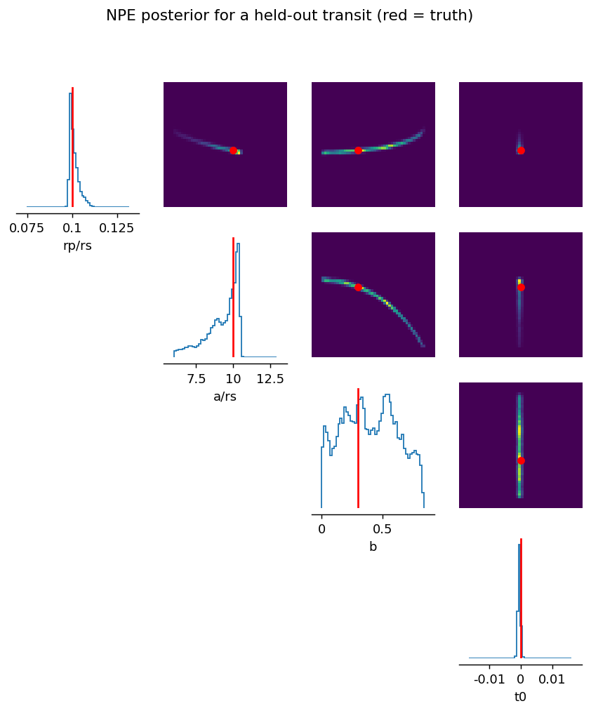
The radius ratio and the transit time come out tight. The impact parameter is barely constrained, and a/rs is broader than the other two. That is not the network failing, it is real physics. A transit shape constrains the combination of a/rs and b much better than either one alone, which is why the corner plot shows those curved ridges instead of round blobs. A point estimate would have hidden that. The posterior shows it directly.
Calibration is the part that matters
A posterior that looks pretty can still be wrong. If it is systematically too narrow, you will report planets with error bars that are too small to trust. Simulation-based calibration is the check. Draw parameters from the prior, simulate data, infer a posterior for each, and record the rank of the true value among the posterior samples. If the posterior is calibrated, those ranks are uniform.
ranks, _ = run_sbc(theta_sbc, x_sbc, posterior, num_posterior_samples=1000)
sbc_rank_plot(ranks, num_posterior_samples=1000, plot_type="hist")
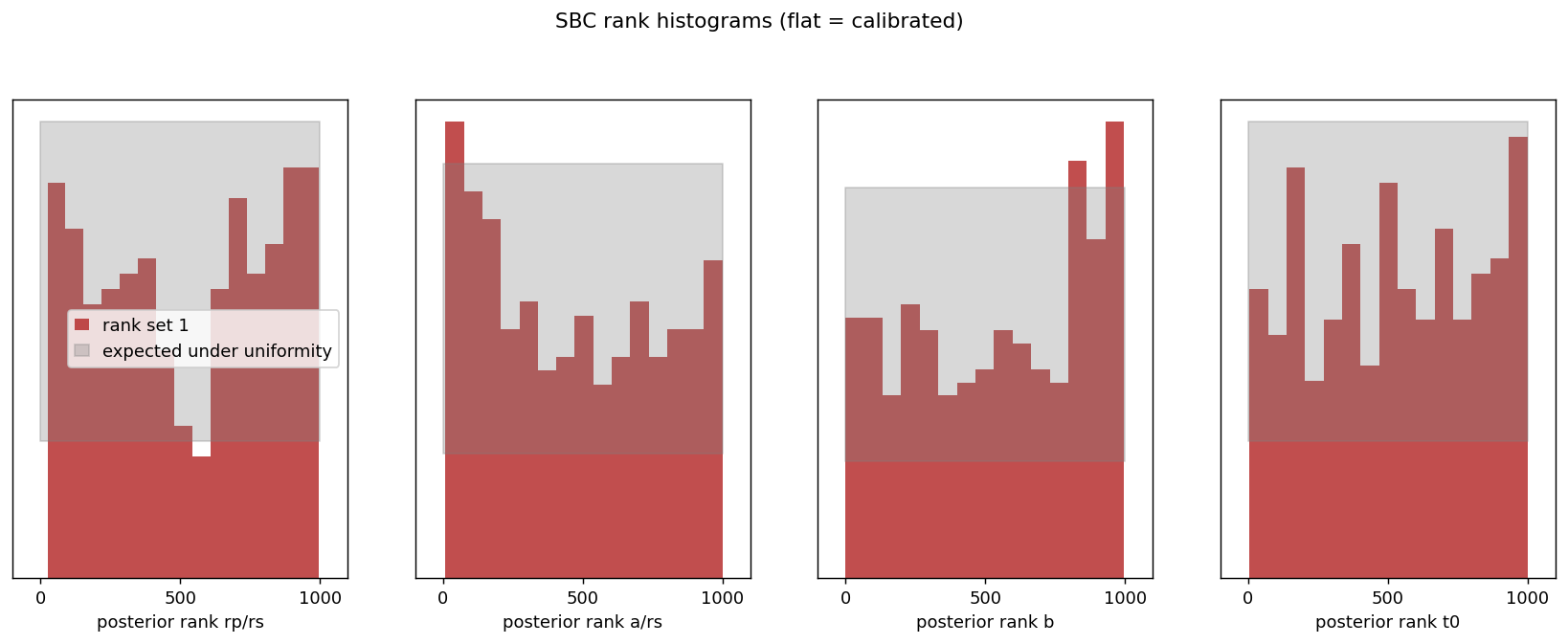
The histograms mostly stay inside the gray band. There are mild deviations: a faint U-shape in rp/rs that hints at slightly over-confident intervals, and a small slope in a/rs and b. With only 8000 training simulations and 300 calibration draws, that is about what you expect, and the cure is more simulations rather than a different method. The point is that you can see the problem at all. A miscalibrated posterior that you never check is far worse than a slightly wide one that you do.
Why I care
This is the machinery from my master’s work in a clean, self-contained form. The same pattern, simulate, train a flow, then prove it is calibrated, carries over to harder problems where the simulator is an N-body or radiative-transfer code and MCMC is hopeless. It is also the kind of modular, documented component I want in a flight-ready portfolio, where “trust the error bars” is not optional. The next post takes the opposite view of the same data: instead of characterizing a known transit, it asks whether a candidate is a planet at all.
Full code
#!/usr/bin/env python
"""Simulation-based inference for exoplanet transits.

Train a neural posterior on synthetic Mandel-Agol transits with sbi, recover
parameters of a held-out transit, and check calibration with simulation-based
calibration (SBC).
"""
import numpy as np
import torch
import torch.nn as nn
import matplotlib.pyplot as plt
import batman
from sbi.inference import NPE
from sbi.neural_nets import posterior_nn
from sbi.utils import BoxUniform
from sbi.analysis import pairplot

torch.manual_seed(0)
np.random.seed(0)

# ---------------------------------------------------------------------------
# simulator: a single transit, 4 free parameters
#   theta = [rp/rs, a/rs, b (impact param), t0]
# limb darkening and period are fixed and known.
# ---------------------------------------------------------------------------
N_TIME = 200
T = np.linspace(-0.15, 0.15, N_TIME)
PERIOD = 5.0
U_LD = [0.3, 0.2]
NOISE = 7e-4
LABELS = ["rp/rs", "a/rs", "b", "t0"]

_pm = batman.TransitParams()
_pm.per = PERIOD
_pm.ecc = 0.0
_pm.w = 90.0
_pm.limb_dark = "quadratic"
_pm.u = U_LD


def simulate_one(theta):
    rp, a, b, t0 = [float(v) for v in theta]
    _pm.rp = rp
    _pm.a = a
    _pm.t0 = t0
    _pm.inc = np.degrees(np.arccos(np.clip(b / a, 0, 1)))
    m = batman.TransitModel(_pm, T)
    flux = m.light_curve(_pm)
    flux = flux + np.random.normal(0, NOISE, N_TIME)
    return flux.astype(np.float32)


def simulator(theta_batch):
    theta_batch = np.atleast_2d(np.asarray(theta_batch))
    return torch.tensor(np.stack([simulate_one(t) for t in theta_batch]))


prior = BoxUniform(
    low=torch.tensor([0.05, 6.0, 0.0, -0.03]),
    high=torch.tensor([0.15, 14.0, 0.9, 0.03]),
)

# ---------------------------------------------------------------------------
# training data
# ---------------------------------------------------------------------------
N_SIM = 8000
theta = prior.sample((N_SIM,))
print(f"[sbi] simulating {N_SIM} transits ...")
x = simulator(theta)
print(f"[sbi] x shape {tuple(x.shape)}")


# ---------------------------------------------------------------------------
# 1D CNN embedding: compress the light curve before the flow
# ---------------------------------------------------------------------------
class CNNEmbed(nn.Module):
    def __init__(self, n_time, out_dim=16):
        super().__init__()
        self.net = nn.Sequential(
            nn.Unflatten(1, (1, n_time)),
            nn.Conv1d(1, 16, 7, padding=3), nn.ReLU(), nn.MaxPool1d(2),
            nn.Conv1d(16, 32, 5, padding=2), nn.ReLU(), nn.MaxPool1d(2),
            nn.Flatten(),
            nn.LazyLinear(out_dim), nn.ReLU(),
        )

    def forward(self, x):
        return self.net(x)


density_estimator = posterior_nn(model="nsf", embedding_net=CNNEmbed(N_TIME))
inference = NPE(prior=prior, density_estimator=density_estimator)
inference.append_simulations(theta, x)
print("[sbi] training neural posterior ...")
inference.train()
posterior = inference.build_posterior()

# ---------------------------------------------------------------------------
# inference on a held-out transit
# ---------------------------------------------------------------------------
theta_true = torch.tensor([0.10, 10.0, 0.3, 0.0])
x_obs = simulator(theta_true.unsqueeze(0))[0]
samples = posterior.sample((20000,), x=x_obs)

med = samples.median(0).values
lo = samples.quantile(0.16, 0)
hi = samples.quantile(0.84, 0)
print("[sbi] parameter recovery (truth -> median [16-84%]):")
for i, name in enumerate(LABELS):
    print(f"  {name:6s} {theta_true[i]:+.4f} -> {med[i]:+.4f} "
          f"[{lo[i]:+.4f}, {hi[i]:+.4f}]")

fig, axes = pairplot(
    samples,
    points=theta_true.unsqueeze(0),
    labels=LABELS,
    points_colors="red",
    figsize=(8, 8),
)
fig.suptitle("NPE posterior for a held-out transit (red = truth)", y=1.0)
fig.savefig("uploads/2026/06/sbi-transit-posterior.png", dpi=130, bbox_inches="tight")
print("[sbi] saved uploads/2026/06/sbi-transit-posterior.png")

# ---------------------------------------------------------------------------
# calibration: simulation-based calibration
# ---------------------------------------------------------------------------
from sbi.diagnostics import run_sbc
from sbi.analysis import sbc_rank_plot

N_SBC = 300
theta_sbc = prior.sample((N_SBC,))
x_sbc = simulator(theta_sbc)
print(f"[sbi] running SBC on {N_SBC} draws ...")
ranks, _ = run_sbc(theta_sbc, x_sbc, posterior, num_posterior_samples=1000)

f, ax = sbc_rank_plot(ranks, num_posterior_samples=1000, plot_type="hist",
                      parameter_labels=LABELS)
fig2 = f if isinstance(f, plt.Figure) else plt.gcf()
fig2.suptitle("SBC rank histograms (flat = calibrated)", y=1.02)
fig2.savefig("uploads/2026/06/sbi-transit-sbc.png", dpi=130, bbox_inches="tight")
print("[sbi] saved uploads/2026/06/sbi-transit-sbc.png")