Radio frequency interference is the main reason technosignature searches drown in false positives. A wide survey returns millions of candidate signals, and almost all of them are satellites, phones, radar or aircraft. The usual fix is a supervised classifier, but that needs you to enumerate the RFI types ahead of time, and the environment keeps changing, so the labels are never complete.
A more honest framing is anomaly detection. Most of what you see is RFI, the interesting signal is rare, so learn what “common” looks like and flag whatever does not fit. This post builds a small β-VAE that does exactly that on spectrogram tiles. It follows the same idea as the recent Breakthrough Listen work, where a β-VAE trained on energy-detector hits cut the false-positive rate by about 99% while keeping nearly all of the real signal.
Why a VAE instead of a classifier
A classifier needs labeled RFI classes. An autoencoder does not. Train it to reconstruct ordinary RFI through a tight bottleneck, and it learns the manifold of “normal”. Anything it reconstructs badly is, by definition, unlike what it was trained on. The β in a β-VAE controls how hard the latent space is squeezed toward a clean prior, which keeps the bottleneck honest.
Synthetic spectrograms
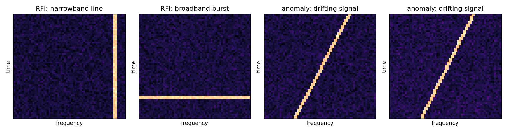
To keep the demo self-contained I generate 64x64 spectrogram tiles. Ordinary RFI is one axis-aligned streak: a vertical narrowband line or a horizontal broadband burst, on a noisy background. The anomaly, which the model never sees in training, is a drifting narrowband signal: a diagonal streak, the Doppler-drifted shape a real technosignature would have.
def add_line(t, orientation):
    amp, w = rng.uniform(0.6, 0.85), 2
    if orientation == "v":      t[:, c:c + w] += amp      # narrowband line
    elif orientation == "h":    t[r:r + w, :] += amp      # broadband burst
    else:                       # diagonal: a drifting signal
        for r in range(S):
            t[r, c(r):c(r) + w] += amp
All three streaks cover the same number of bright pixels, so the classes differ in structure, not in brightness. That detail matters. An earlier version had thin diagonals with less total energy, and the reconstruction error happily flagged them for the wrong reason, scoring dim tiles as anomalies regardless of shape.
The model
A convolutional β-VAE with an 8-dimensional latent, trained only on RFI tiles.
def loss_fn(x, xh, mu, lv, beta):
    recon = F.mse_loss(xh, x, reduction="sum") / x.shape[0]
    kld = -0.5 * torch.sum(1 + lv - mu.pow(2) - lv.exp()) / x.shape[0]
    return recon + beta * kld
I trained on 6000 RFI tiles for 50 epochs, a few seconds on the laptop GPU. The anomaly score for any tile is just its reconstruction error.
It works, and you can see why
On a test set of 1000 RFI tiles and 200 drifting-signal anomalies:
mean recon error  RFI=0.0016  anomaly=0.0177
anomaly-detection ROC AUC = 1.0000
keeping 95% of anomalies cuts 100.0% of the RFI
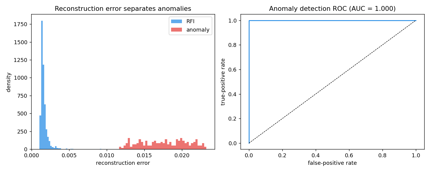
The error on a drifting signal is about eleven times the error on RFI. The reason is visible if you look at what the decoder actually produces.
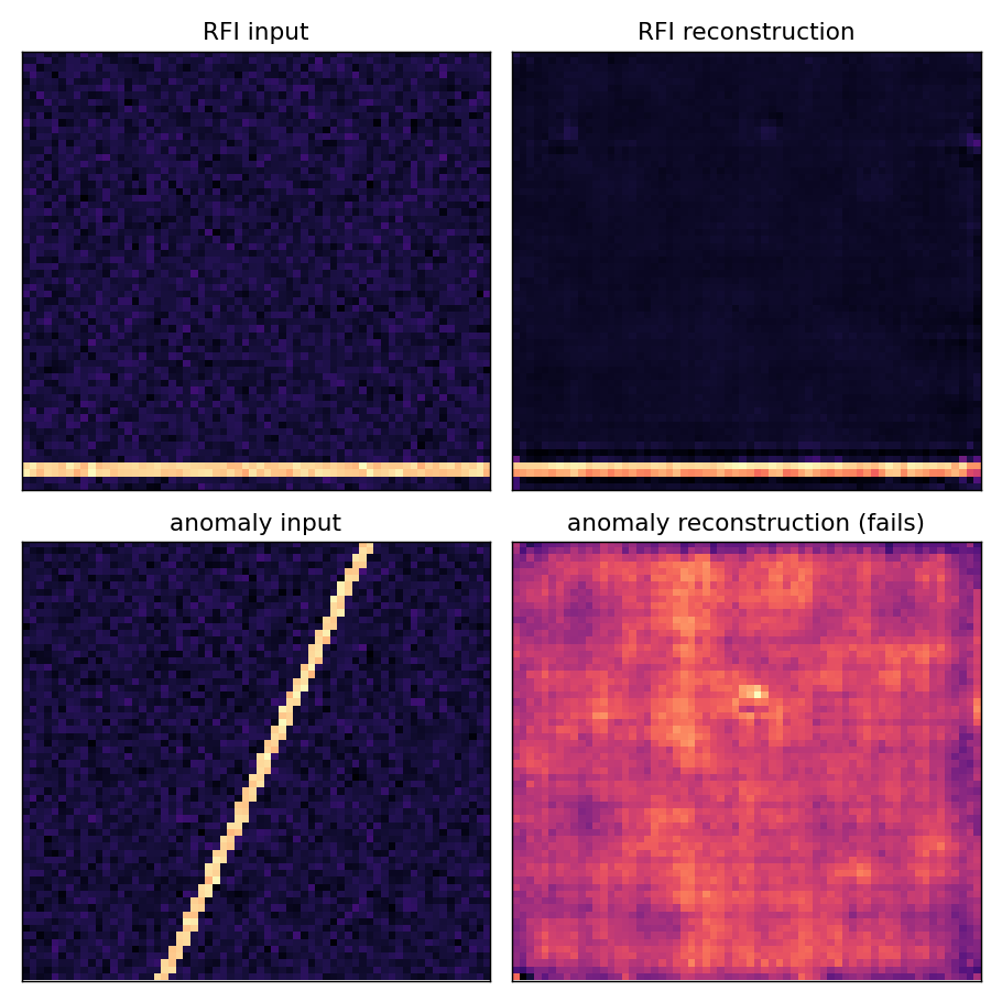
The decoder learned to paint axis-aligned lines and nothing else. Hand it a diagonal and the best it can do is a confused blur, which leaves a large residual. That residual is the signal.
A note on the choice of network. I first tried this with a wider latent and it failed, because a roomy convolutional decoder happily generalizes to diagonals and reconstructs the anomaly almost as well as the RFI. The detector only works when the bottleneck is tight enough that the unfamiliar structure genuinely cannot pass through it. The constraint is the point, not an inconvenience.
Honest limits
The perfect separation here is a property of clean synthetic data with exactly two normal orientations. Real RFI is far more varied, the normal manifold is much larger, and you have to train on the actual RFI environment of your telescope, which keeps shifting as new satellite constellations go up. That is why the real-world result is a strong reduction rather than a clean cut. The mechanism is the same though: the model triages, dropping the haystack by orders of magnitude so a person reviews hundreds of candidates instead of millions. And anomaly detection finds anything unusual, not aliens specifically. A new kind of RFI scores just as high as a real signal. The output is a shortlist, not a discovery. This is the stage that sits right after the matched filter in the pipeline, and it is the part of the SETI search I find most interesting to work on.
Full code
#!/usr/bin/env python
"""Killing RFI with a beta-VAE.

Train a beta-VAE on synthetic spectrogram tiles containing only ordinary RFI
(narrowband lines, broadband bursts). At test time, score tiles by
reconstruction error. Drifting narrowband signals -- the technosignature-like
case the model never saw -- reconstruct badly and stand out as anomalies.
"""
import numpy as np
import torch
import torch.nn as nn
import matplotlib.pyplot as plt
from sklearn.metrics import roc_auc_score, roc_curve

rng = np.random.default_rng(3)
torch.manual_seed(0)
device = "mps" if torch.backends.mps.is_available() else "cpu"
S = 64  # tile size (time x frequency)


# ---------------------------------------------------------------------------
# synthetic spectrogram tiles
# ---------------------------------------------------------------------------
def background():
    return rng.normal(0.10, 0.03, (S, S)).clip(0, 1).astype(np.float32)


def add_line(t, orientation):
    """Add one bright streak. All orientations cover ~S pixels at the same
    brightness, so the classes differ in structure, not in total energy."""
    amp = rng.uniform(0.6, 0.85)
    w = 2
    if orientation == "v":                       # narrowband line (vertical)
        c = rng.integers(0, S - w)
        t[:, c:c + w] += amp
    elif orientation == "h":                     # broadband burst (horizontal)
        r = rng.integers(0, S - w)
        t[r:r + w, :] += amp
    else:                                        # drifting signal (diagonal)
        # keep the streak in-frame so it spans all S rows, matching the pixel
        # count of an axis-aligned line.
        # drifts range from shallow (looks almost like a vertical RFI line, the
        # hardest case) to steep.
        drift = rng.uniform(0.1, 0.7) * (1 if rng.random() < 0.5 else -1)
        f0 = S / 2 - drift * S / 2
        for r in range(S):
            c = int(round(f0 + drift * r))
            c = min(max(c, 0), S - w)
            t[r, c:c + w] += amp


def rfi_tile():
    """Ordinary RFI: one axis-aligned line (vertical or horizontal)."""
    t = background()
    add_line(t, "v" if rng.random() < 0.5 else "h")
    return t.clip(0, 1)


def anomaly_tile():
    """A drifting narrowband signal: one diagonal streak the model never saw."""
    t = background()
    add_line(t, "d")
    return t.clip(0, 1)


def batch(n, fn):
    return np.stack([fn() for _ in range(n)])[:, None, :, :]


print("[vae] building tiles ...")
Xtr = torch.tensor(batch(6000, rfi_tile), device=device)
Xte_rfi = batch(1000, rfi_tile)
Xte_anom = batch(200, anomaly_tile)
Xte = torch.tensor(np.concatenate([Xte_rfi, Xte_anom]), device=device)
yte = np.concatenate([np.zeros(1000), np.ones(200)])  # 1 = anomaly


# ---------------------------------------------------------------------------
# beta-VAE
# ---------------------------------------------------------------------------
class BetaVAE(nn.Module):
    """Convolutional beta-VAE with a tight 8-dim latent. Trained only on
    axis-aligned lines, its decoder learns to paint that narrow family well,
    so an unfamiliar diagonal falls off the learned manifold and reconstructs
    badly. That gap in reconstruction error is the anomaly score."""

    def __init__(self, latent=8, beta=0.5):
        super().__init__()
        self.beta = beta
        self.enc = nn.Sequential(
            nn.Conv2d(1, 16, 4, 2, 1), nn.ReLU(),    # 64 -> 32
            nn.Conv2d(16, 32, 4, 2, 1), nn.ReLU(),   # 32 -> 16
            nn.Conv2d(32, 64, 4, 2, 1), nn.ReLU(),   # 16 -> 8
            nn.Flatten())
        self.fc_mu = nn.Linear(64 * 8 * 8, latent)
        self.fc_lv = nn.Linear(64 * 8 * 8, latent)
        self.fc_dec = nn.Linear(latent, 64 * 8 * 8)
        self.dec = nn.Sequential(
            nn.Unflatten(1, (64, 8, 8)),
            nn.ConvTranspose2d(64, 32, 4, 2, 1), nn.ReLU(),
            nn.ConvTranspose2d(32, 16, 4, 2, 1), nn.ReLU(),
            nn.ConvTranspose2d(16, 1, 4, 2, 1), nn.Sigmoid())

    def forward(self, x):
        h = self.enc(x)
        mu, lv = self.fc_mu(h), self.fc_lv(h)
        z = mu + torch.randn_like(mu) * torch.exp(0.5 * lv)
        return self.dec(self.fc_dec(z)), mu, lv


def loss_fn(x, xh, mu, lv, beta):
    recon = nn.functional.mse_loss(xh, x, reduction="sum") / x.shape[0]
    kld = -0.5 * torch.sum(1 + lv - mu.pow(2) - lv.exp()) / x.shape[0]
    return recon + beta * kld


vae = BetaVAE().to(device)
opt = torch.optim.Adam(vae.parameters(), lr=1e-3)
print(f"[vae] training on {device} ...")
for epoch in range(50):
    vae.train()
    perm = torch.randperm(len(Xtr), device=device)
    for i in range(0, len(Xtr), 128):
        b = Xtr[perm[i:i + 128]]
        opt.zero_grad()
        xh, mu, lv = vae(b)
        loss = loss_fn(b, xh, mu, lv, vae.beta)
        loss.backward()
        opt.step()


# ---------------------------------------------------------------------------
# anomaly score = per-tile reconstruction error
# ---------------------------------------------------------------------------
@torch.no_grad()
def recon_error(X):
    vae.eval()
    errs = []
    for i in range(0, len(X), 256):
        b = X[i:i + 256]
        xh, _, _ = vae(b)
        errs.append(((xh - b) ** 2).mean(dim=(1, 2, 3)).cpu().numpy())
    return np.concatenate(errs)


scores = recon_error(Xte)
auc = roc_auc_score(yte, scores)
rfi_err, anom_err = scores[yte == 0], scores[yte == 1]
print(f"[vae] mean recon error  RFI={rfi_err.mean():.4f}  anomaly={anom_err.mean():.4f}")
print(f"[vae] anomaly-detection ROC AUC = {auc:.4f}")
# how much of the haystack we can cut while keeping 95% of anomalies
thr95 = np.quantile(anom_err, 0.05)
cut = (rfi_err < thr95).mean()
print(f"[vae] keeping 95% of anomalies cuts {cut:.1%} of the RFI")

# ---------------------------------------------------------------------------
# figure 1: example tiles
# ---------------------------------------------------------------------------
def forced(orient):
    t = background(); add_line(t, orient); return t.clip(0, 1)


fig, ax = plt.subplots(1, 4, figsize=(13, 3.4))
ax[0].imshow(forced("v"), aspect="auto", cmap="magma"); ax[0].set_title("RFI: narrowband line")
ax[1].imshow(forced("h"), aspect="auto", cmap="magma"); ax[1].set_title("RFI: broadband burst")
ax[2].imshow(anomaly_tile(), aspect="auto", cmap="magma"); ax[2].set_title("anomaly: drifting signal")
ax[3].imshow(anomaly_tile(), aspect="auto", cmap="magma"); ax[3].set_title("anomaly: drifting signal")
for a in ax:
    a.set_xlabel("frequency"); a.set_ylabel("time"); a.set_xticks([]); a.set_yticks([])
fig.tight_layout()
fig.savefig("uploads/2026/06/rfi-vae-examples.png", dpi=130)
print("[vae] saved uploads/2026/06/rfi-vae-examples.png")

# ---------------------------------------------------------------------------
# figure 2: score histogram + ROC
# ---------------------------------------------------------------------------
fig2, ax2 = plt.subplots(1, 2, figsize=(11, 4.4))
ax2[0].hist(rfi_err, bins=40, alpha=0.7, color="#1e88e5", label="RFI", density=True)
ax2[0].hist(anom_err, bins=40, alpha=0.7, color="#e53935", label="anomaly", density=True)
ax2[0].set_xlabel("reconstruction error"); ax2[0].set_ylabel("density")
ax2[0].set_title("Reconstruction error separates anomalies"); ax2[0].legend()

fpr, tpr, _ = roc_curve(yte, scores)
ax2[1].plot(fpr, tpr, color="#1e88e5")
ax2[1].plot([0, 1], [0, 1], "k--", lw=0.8)
ax2[1].set_xlabel("false-positive rate"); ax2[1].set_ylabel("true-positive rate")
ax2[1].set_title(f"Anomaly detection ROC (AUC = {auc:.3f})")
fig2.tight_layout()
fig2.savefig("uploads/2026/06/rfi-vae-scores.png", dpi=130)
print("[vae] saved uploads/2026/06/rfi-vae-scores.png")

# ---------------------------------------------------------------------------
# figure 3: input vs reconstruction, normal RFI vs anomaly
# ---------------------------------------------------------------------------
@torch.no_grad()
def recon(x_np):
    vae.eval()
    x = torch.tensor(x_np[None, None], device=device)
    xh, _, _ = vae(x)
    return xh[0, 0].cpu().numpy()


norm_in = rfi_tile().astype(np.float32)
anom_in = anomaly_tile().astype(np.float32)
fig3, ax3 = plt.subplots(2, 2, figsize=(7, 7))
for a, img, title in [
    (ax3[0, 0], norm_in, "RFI input"),
    (ax3[0, 1], recon(norm_in), "RFI reconstruction"),
    (ax3[1, 0], anom_in, "anomaly input"),
    (ax3[1, 1], recon(anom_in), "anomaly reconstruction (fails)")]:
    a.imshow(img, aspect="auto", cmap="magma"); a.set_title(title)
    a.set_xticks([]); a.set_yticks([])
fig3.tight_layout()
fig3.savefig("uploads/2026/06/rfi-vae-reconstructions.png", dpi=130)
print("[vae] saved uploads/2026/06/rfi-vae-reconstructions.png")