In Dedispersion I wrote about undoing the frequency sweep that plasma adds to a pulse. Dedispersion gets the energy lined up in time, but it does not tell you whether a pulse is actually there. That second step is a detection problem, and the best linear tool for it is the matched filter.
This post derives the matched filter from the detection problem and then runs it against a pulse buried in noise, so the derivation and the run end up agreeing.
The detection problem
You have a time series $x(t)$ and you want to choose between two cases:
\[\begin{aligned} H_0 &: x(t) = n(t) \\ H_1 &: x(t) = s(t) + n(t) \end{aligned}\]Here $s(t)$ is a signal of known shape and $n(t)$ is noise. The signal might be a dedispersed pulse; the noise is the radiometer noise of the system. The question is which linear filter $h$ gives the largest signal-to-noise ratio at its output.
Why the optimal filter is the signal itself, reversed
Pass $x$ through a filter $h$ and read the output at the instant the pulse should peak. Its signal part is the inner product of $h$ with $s$, while the noise part has variance set by the energy of $h$ times the noise level. So the quantity to maximize is
\[\text{SNR} \propto \frac{\langle h, s \rangle}{\lVert h \rVert}\]The Cauchy-Schwarz inequality says an inner product divided by the norm of one vector is largest when that vector points along the other one. So the best filter is a scaled copy of the signal, time-reversed for the convolution:
\[h(t) \propto s(-t)\]That is the whole idea. The optimal detector for a known shape is that same shape, used as a correlation template. When the noise is not white but has power spectral density $N(\nu)$, the filter picks up a whitening factor:
\[H(\nu) = \frac{S^*(\nu)}{N(\nu)}\]which is the form used in gravitational-wave and FRB pipelines, where the noise is strongly colored.
Implementation
The white-noise version is a few lines. np.correlate already time-reverses the template, so the only extra step is normalizing the template to unit energy, which puts the output directly in SNR units.
import numpy as np

def matched_filter(x, template):
    t = template / np.linalg.norm(template)
    return np.correlate(x, t, mode="same")
To test it, I inject a Gaussian pulse of peak amplitude 1.2 into white noise of unit standard deviation, at sample 2600. With a per-sample amplitude close to the noise level, the pulse is invisible in the raw series.
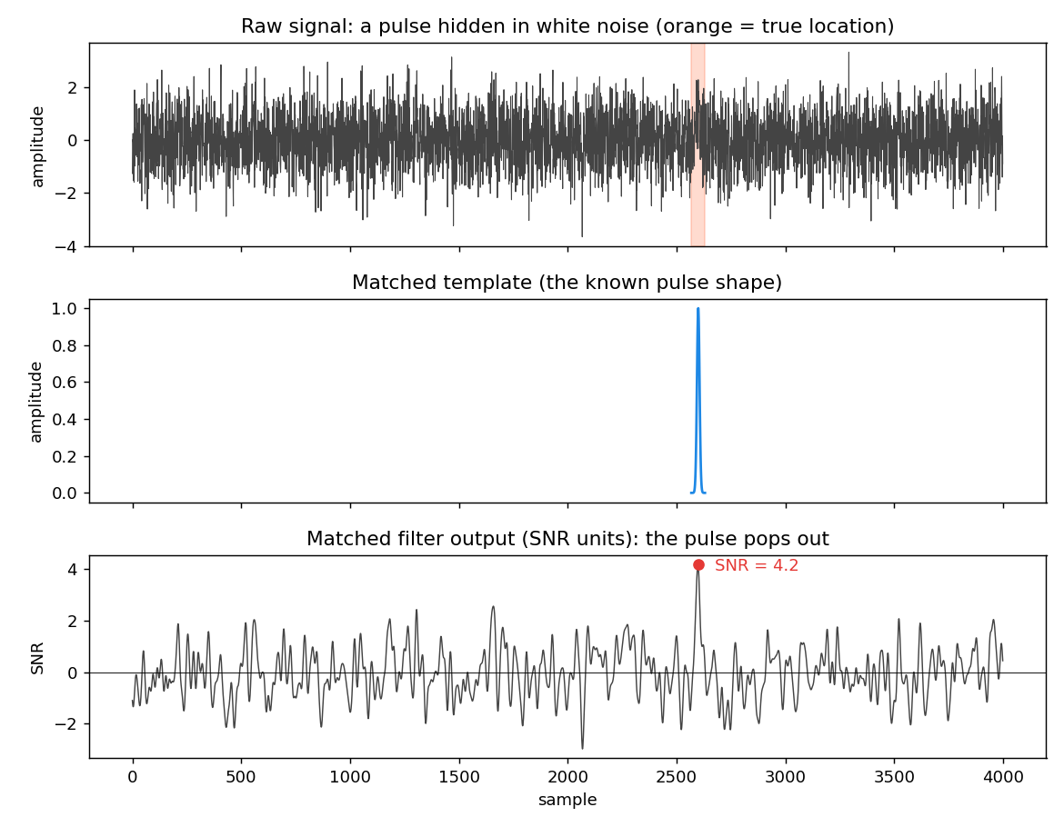
The filter recovers the pulse at sample 2599, one sample off the injection point, at an output SNR of 4.2. Nothing else in the record comes close. The pulse you could not see by eye is an unambiguous peak after filtering.
The pulse width is usually unknown
In a real single-pulse search you do not know the width of the pulse in advance. A matched filter tuned to the wrong width loses SNR, so pipelines run a bank of boxcar filters at a range of widths and keep the width that gives the strongest response.
widths = np.arange(1, 41)
recovered_snr = [np.max(matched_filter(x, np.ones(w))) / sigma
                 for w in widths]
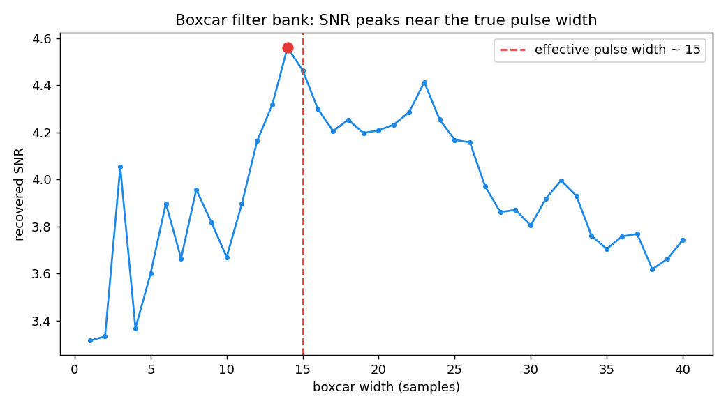
The Gaussian pulse has an effective width of about 15 samples, and the boxcar bank peaks at width 14. A boxcar is a crude stand-in for a Gaussian, so the recovered SNR is a little below the matched case, which is the price of not knowing the exact shape. This is the same trade that drives the width trials in FRB and pulsar search software.
Where it breaks
The derivation assumes a known signal shape and stationary noise. Real data violates both. The pulse shape drifts with scattering and instrument response, and the noise is anything but stationary once radio frequency interference enters. RFI shows up as short, bright, FRB-like bursts that a boxcar bank happily flags, which is exactly why dedispersion and matched filtering alone are not enough. That false-positive problem is the subject of the next post, where the filter bank hands off to a learned RFI rejector.
Full code
#!/usr/bin/env python
"""Matched filtering from scratch.

Injects a known pulse into white noise, recovers it with a matched filter,
then sweeps a bank of boxcar widths to show why pulse-search pipelines use a
filter bank. Produces two figures.
"""
import numpy as np
import matplotlib.pyplot as plt

rng = np.random.default_rng(20260608)

# ---------------------------------------------------------------------------
# core
# ---------------------------------------------------------------------------
def matched_filter(x, template):
    """Correlate x with a unit-energy, time-reversed template.

    np.correlate already does the time reversal, so we just normalize the
    template to unit energy. With white noise of variance sigma^2 the output
    at the true location has expected SNR = ||s|| / sigma.
    """
    t = template / np.linalg.norm(template)
    return np.correlate(x, t, mode="same")


def gaussian_pulse(width, n=64):
    t = np.arange(n) - n / 2
    p = np.exp(-0.5 * (t / width) ** 2)
    return p / p.max()


# ---------------------------------------------------------------------------
# figure 1: detection of a single pulse buried in noise
# ---------------------------------------------------------------------------
N = 4000
sigma = 1.0
amp = 1.2                 # peak amplitude -- comparable to the noise sigma
true_width = 6.0
loc = 2600               # sample index where the pulse is injected

pulse = amp * gaussian_pulse(true_width, n=64)
x = rng.normal(0, sigma, N)
x[loc - 32:loc + 32] += pulse

template = gaussian_pulse(true_width, n=64)
y = matched_filter(x, template)

# theoretical noise level at the filter output is sigma (template is unit energy)
snr = y / sigma
peak = int(np.argmax(snr))

print(f"[fig1] injected at {loc}, detected at {peak} (off by {peak - loc})")
print(f"[fig1] peak SNR = {snr[peak]:.2f}")

fig, ax = plt.subplots(3, 1, figsize=(9, 7), sharex=True)
ax[0].plot(x, lw=0.6, color="#444")
ax[0].axvspan(loc - 32, loc + 32, color="#ff7043", alpha=0.25)
ax[0].set_title("Raw signal: a pulse hidden in white noise (orange = true location)")
ax[0].set_ylabel("amplitude")

tt = np.arange(64) + loc - 32
ax[1].plot(tt, template, color="#1e88e5")
ax[1].set_title("Matched template (the known pulse shape)")
ax[1].set_ylabel("amplitude")

ax[2].plot(snr, lw=0.8, color="#444")
ax[2].axhline(0, color="k", lw=0.5)
ax[2].plot(peak, snr[peak], "o", color="#e53935")
ax[2].annotate(f"SNR = {snr[peak]:.1f}", (peak, snr[peak]),
               textcoords="offset points", xytext=(10, -4), color="#e53935")
ax[2].set_title("Matched filter output (SNR units): the pulse pops out")
ax[2].set_ylabel("SNR")
ax[2].set_xlabel("sample")
fig.tight_layout()
fig.savefig("uploads/2026/06/matched-filter-detection.png", dpi=130)
print("[fig1] saved uploads/2026/06/matched-filter-detection.png")

# ---------------------------------------------------------------------------
# figure 2: boxcar filter bank -- the pulse width is unknown in practice
# ---------------------------------------------------------------------------
# a real single-pulse search does not know the pulse width, so it runs a bank
# of boxcar matched filters and keeps the width that maximizes SNR.
widths = np.arange(1, 41)
recovered_snr = []
for w in widths:
    boxcar = np.ones(w)
    yb = matched_filter(x, boxcar)
    recovered_snr.append(np.max(yb) / sigma)
recovered_snr = np.array(recovered_snr)
best_w = widths[int(np.argmax(recovered_snr))]

# the gaussian pulse has an effective width ~ sqrt(2*pi)*true_width samples
eff_width = np.sqrt(2 * np.pi) * true_width
print(f"[fig2] best boxcar width = {best_w}, effective pulse width ~ {eff_width:.1f}")

fig2, ax2 = plt.subplots(figsize=(8, 4.5))
ax2.plot(widths, recovered_snr, "-o", ms=3, color="#1e88e5")
ax2.axvline(eff_width, color="#e53935", ls="--",
            label=f"effective pulse width ~ {eff_width:.0f}")
ax2.plot(best_w, recovered_snr.max(), "o", color="#e53935", ms=8)
ax2.set_xlabel("boxcar width (samples)")
ax2.set_ylabel("recovered SNR")
ax2.set_title("Boxcar filter bank: SNR peaks near the true pulse width")
ax2.legend()
fig2.tight_layout()
fig2.savefig("uploads/2026/06/matched-filter-boxcar-bank.png", dpi=130)
print("[fig2] saved uploads/2026/06/matched-filter-boxcar-bank.png")