The most interesting SETI software may not be the first detector. It may be the system that handles what happens after a candidate appears.
Working around radio data made me care less about the dramatic first detection and more about what happens in the next ten minutes. Can I find the raw file? Can I rebuild the processing step? Was the telescope really on target? Was a satellite crossing the beam? Did the same thing appear off-source? Is the signal simply a transmitter we already know?
I tested that idea with a real HDF5 observation of Voyager 1. It is not an unknown SETI candidate, and that is exactly why it is useful. Voyager gives me a strong, narrowband, real transmitter with real metadata. A post-detection pipeline has to represent it, preserve provenance, classify it as known, and produce a small report without pretending it found anything mysterious.
The data I used
The file was already on my machine:
~/Workspace/SRC/Python/ASTRO/SETI/0/Voyager1.single_coarse.fine_res.h5
For replication, the same file is available from the Breakthrough Listen public data server:
http://blpd0.ssl.berkeley.edu/Voyager_data/Voyager1.single_coarse.fine_res.h5
The note beside my local copy points to a Voyager/turboSETI machine-learning demo. I also checked the blimpy Voyager notebook, which uses the same public HDF5 file to demonstrate Breakthrough Listen filterbank data. For this post I did not use a neural network. I only needed the HDF5 data product and its metadata.
I inspected it with h5py in the exohunter conda environment. The file uses an HDF5 compression plugin, so the important detail is importing hdf5plugin before reading the dataset:
import hdf5plugin
import h5py
import numpy as np

path = "Voyager1.single_coarse.fine_res.h5"

with h5py.File(path, "r") as f:
    data = np.squeeze(f["data"][...])
    attrs = dict(f["data"].attrs)
After removing the feed axis, the array was:
16 integrations x 1,048,576 frequency channels
The metadata was already enough to build a candidate record:
source_name: Voyager1
rawdatafile: guppi_57650_67573_Voyager1_0002.0000.raw
tstart: 57650.78209490741 MJD
tsamp: 18.253611008 s
fch1: 8421.386717353016 MHz
foff: -2.7939677238464355 Hz/channel
That is already a post-detection lesson. The signal is not only a bright line in an image. It is tied to a source name, raw file, start time, sampling interval, frequency axis, and software path. Without those, the candidate is just a screenshot.
The extraction script
I put the extraction code in:
res/post_detection_seti_voyager.py
I ran it with:
MPLCONFIGDIR=/tmp/mplconfig \
conda run -n exohunter python res/post_detection_seti_voyager.py \
  /Users/paolo/Workspace/SRC/Python/ASTRO/SETI/0/Voyager1.single_coarse.fine_res.h5 \
  --plot uploads/2026/06/voyager1-post-detection-candidate.png \
  --json /tmp/voyager1-post-detection-candidate.json
The script does a deliberately simple extraction: find the strongest channel in each integration, convert the channel index to frequency, fit a line to frequency over time, compute a robust S/N-like score, hash the input file, and save a waterfall cutout around the peak.
There is one trap in this file: the strongest feature in the full coarse channel is the central DC bin, an FFT artifact. The blimpy Voyager notebook points this out before zooming into Voyager’s telemetry around 8419.296-8419.298 MHz. I used that same carrier window instead of blindly taking the global maximum.
That mistake is worth making once. My first extraction did exactly the wrong thing: it found the largest value in the whole file and locked onto the DC bin at the middle of the coarse channel. The plot looked dramatic, but it was not the Voyager carrier. This is the whole post-detection problem in miniature: maximum power is not the same as a meaningful candidate.
fch1_mhz = float(attrs["fch1"])
foff_mhz = float(attrs["foff"])
tsamp_s = float(attrs["tsamp"])

freq_axis_mhz = fch1_mhz + np.arange(data.shape[1]) * foff_mhz
search = (freq_axis_mhz >= 8419.296) & (freq_axis_mhz <= 8419.298)

search_ch = np.arange(data.shape[1])[search]
sub = data[:, search]
peak_rel = np.nanargmax(sub, axis=1)
peak_ch = search_ch[peak_rel]
peak_val = data[np.arange(data.shape[0]), peak_ch]

peak_freq_mhz = fch1_mhz + peak_ch * foff_mhz
time_s = np.arange(data.shape[0]) * tsamp_s
drift_hz_s = np.polyfit(time_s, peak_freq_mhz * 1e6, 1)[0]
The peak was not subtle:
search window: 8419.296-8419.298 MHz
peak channel range: 747929-747966
representative peak frequency: 8419.296977576 MHz
estimated drift: -0.374 Hz/s over this short file
Using a robust median/MAD estimate over the array, the peak was tens of thousands of sigma above the local background:
global median: 1.0655721472e10
robust sigma: 1.452514944e9
peak S/N-like range: 181.48 to 234.32
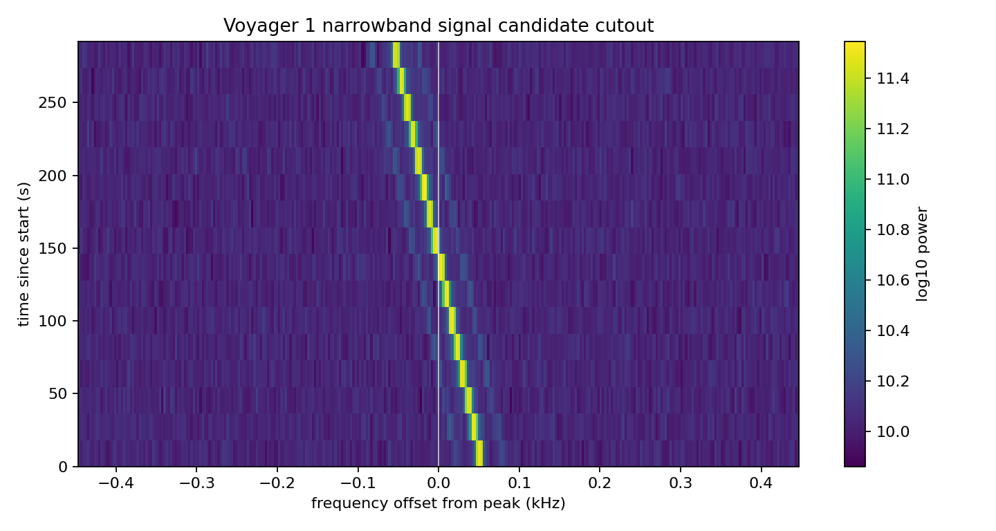
The frequency drift is visible in the cutout, but I also kept the numbers:
time_s    peak_freq_mhz      snr_like
0.000     8419.297027867     205.63
91.268    8419.296994340     217.08
182.536   8419.296960812     234.32
273.804   8419.296924490     181.48
Over this short file, a straight-line fit gives about -0.374 Hz/s. That is the kind of field I want in the candidate record because a narrowband signal without its drift rate is only half described.
The generated candidate record looked like this:
{
  "candidate_id": "voyager1-57650-0001",
  "source_url": "http://blpd0.ssl.berkeley.edu/Voyager_data/Voyager1.single_coarse.fine_res.h5",
  "source_name": "Voyager1",
  "rawdatafile": "guppi_57650_67573_Voyager1_0002.0000.raw",
  "timestamp_mjd": 57650.78209490741,
  "timestamp_utc": "2016-09-19T18:46:13.000",
  "n_integrations": 16,
  "n_channels": 1048576,
  "tsamp_s": 18.253611008,
  "search_f_start_mhz": 8419.296,
  "search_f_stop_mhz": 8419.298,
  "frequency_hz": 8419296977.575869,
  "peak_channel": 747947,
  "peak_channel_min": 747929,
  "peak_channel_max": 747966,
  "drift_hz_s": -0.3741059982862968,
  "snr_like_min": 181.4794921875,
  "snr_like_max": 234.31748962402344,
  "sha256": "c9a9a54f4140e3754ffb2455fae4eeb2eb70c8207123116ee953e4fce15c36ac",
  "status": "known_transmitter"
}
That record is the point of the post. A detector could produce an enormous score here, but the right status is not candidate_of_interest. It is known_transmitter.
What this is not
This is not a new detection. It is not a claim about an unknown signal. It is not a full turboSETI run, and it is not a complete SETI search.
It is a post-detection engineering test using a known transmitter. That keeps the interpretation honest. I know what the signal is, so I can focus on whether the pipeline captures the things that matter after a detector fires: frequency, drift, time, source metadata, file provenance, generated artifacts, and candidate state.
Candidate records are not paperwork
I do not want a detector to output only a score. I want it to output a structured object that another process can inspect:
{
  "candidate_id": "voyager1-57650-0001",
  "timestamp_utc": "2016-09-19T18:46:13.000",
  "source_url": "http://blpd0.ssl.berkeley.edu/Voyager_data/Voyager1.single_coarse.fine_res.h5",
  "source_name": "Voyager1",
  "frequency_hz": 8419296977.575869,
  "drift_hz_s": -0.3741059982862968,
  "snr_like_max": 234.31748962402344,
  "data_product": "Voyager1.single_coarse.fine_res.h5",
  "status": "known_transmitter"
}
The radio-specific fields matter. A narrowband candidate with drift is a different object from a broadband pulse. A candidate seen on-source means something different from the same feature seen everywhere. A candidate tied to Voyager1 is a known spacecraft signal, not a mystery.
Provenance is part of the signal
The hash in the record is not decoration. It says which bytes produced the candidate:
import hashlib


def sha256_file(path):
    h = hashlib.sha256()
    with open(path, "rb") as f:
        for chunk in iter(lambda: f.read(1024 * 1024), b""):
            h.update(chunk)
    return h.hexdigest()
For this run, the HDF5 file hash was:
c9a9a54f4140e3754ffb2455fae4eeb2eb70c8207123116ee953e4fce15c36ac
The hash does not prove that a signal is important. It proves which file was used when I made the plot and the candidate record. If I rerun the analysis later and get a different result, the first question is whether the input bytes changed.
The triage state
For Voyager, the first triage step is easy. The source name and target are already enough to classify the event as a known transmitter:
def classify_known_transmitter(candidate):
    known_sources = {"Voyager1", "Voyager2"}
    if candidate["source_name"] in known_sources:
        return "known_transmitter", "source name matches known spacecraft"
    return None, "no known transmitter match"
For an unknown candidate, the triage would ask different questions:
Was the telescope on target?
Was the receiver healthy?
Was the candidate seen off target?
Was a satellite or aircraft near the beam?
Did the same feature appear in another beam?
Can the raw data be located?
Can the processing version be rebuilt?
These questions do not answer whether the signal is artificial or non-human. They answer whether the candidate is worth treating as a candidate.
On-source and off-source
The on/off-source test is one of the simplest ideas worth preserving in the data model. If a candidate appears while looking at the target and also appears when the telescope points away, the signal is probably local, instrumental, or coming through a sidelobe. It may still be useful as an RFI artifact, but it is not a strong SETI candidate.
If the signal appears only on-source, it survives one filter. That is all. It does not become evidence of non-human technology. It becomes a candidate that deserves the next check.
That distinction is why I keep beam, source_name, and triage history in the record. A final report that says only “S/N 234” is not enough. For Voyager, the high score is exactly what I expect from a known transmitter.
A tiny state machine
The candidate needs a state machine. I used this minimal one:
VALID_TRANSITIONS = {
    "needs_triage": {
        "known_transmitter",
        "rfi_rejected",
        "needs_reobservation",
    },
    "needs_reobservation": {
        "reobserved_missing",
        "reobserved_present",
    },
    "reobserved_present": {"needs_independent_check"},
    "needs_independent_check": {"closed", "escalated"},
}
I also keep every transition as an event:
def transition(candidate, new_status, reason, events):
    allowed = VALID_TRANSITIONS[candidate["status"]]
    if new_status not in allowed:
        raise ValueError(
            f"invalid transition {candidate['status']} -> {new_status}"
        )

    old_status = candidate["status"]
    candidate["status"] = new_status
    events.append({
        "candidate_id": candidate["candidate_id"],
        "old_status": old_status,
        "new_status": new_status,
        "reason": reason,
    })
This looks too formal until the first ambiguous event. Then it becomes useful. A team needs to know who changed the status, why, and which evidence was attached.
For the Voyager record, the transition is boring and correct:
needs_triage -> known_transmitter
reason: source name matches known spacecraft
In a real pipeline, that transition would close the candidate as an unknown SETI event. It might still be useful as a calibration example, a regression test, or a known-signal sanity check, but it would not go to re-observation as a mystery.
A small database shape
For a real pipeline I would not keep this only in memory. A small SQLite schema already makes the boundaries clearer:
CREATE TABLE candidates (
    candidate_id TEXT PRIMARY KEY,
    timestamp_utc TEXT NOT NULL,
    source_name TEXT,
    frequency_hz REAL NOT NULL,
    drift_hz_s REAL,
    snr_like_max REAL,
    data_product TEXT NOT NULL,
    status TEXT NOT NULL
);

CREATE TABLE triage_events (
    id INTEGER PRIMARY KEY AUTOINCREMENT,
    candidate_id TEXT NOT NULL,
    timestamp_utc TEXT NOT NULL,
    old_status TEXT,
    new_status TEXT,
    reason TEXT NOT NULL
);

CREATE TABLE artifacts (
    id INTEGER PRIMARY KEY AUTOINCREMENT,
    candidate_id TEXT NOT NULL,
    artifact_type TEXT NOT NULL,
    uri TEXT NOT NULL,
    sha256 TEXT,
    description TEXT
);
This is not a full observatory archive. It is the minimum shape I want before taking candidates seriously: candidate state, state-change history, and links to the artifacts that support the decision.
Re-observation is another state
Voyager does not need re-observation as an unknown candidate because it is already a known transmitter. For a real unknown, surviving first triage only earns another observation. I represent that as another state transition:
def apply_reobservation(candidate, detected_again, events):
    if candidate["status"] != "needs_reobservation":
        raise ValueError("candidate is not waiting for re-observation")

    if detected_again:
        transition(
            candidate,
            "reobserved_present",
            "candidate-like feature detected in scheduled re-observation",
            events,
        )
    else:
        transition(
            candidate,
            "reobserved_missing",
            "no matching feature detected in scheduled re-observation",
            events,
        )
Most candidates disappear here. That is not disappointing. It is normal. A serious candidate is one that survives repeated attempts to kill it.
Public communication needs state
SETI has a public communication problem built into it. A weak or unverified candidate can spread faster than the verification process. That means the internal state machine and evidence package matter before anyone writes a public sentence.
I would want a candidate report to separate:
what was observed
what has been ruled out
what has not been checked
what would change the status
who reviewed it
what data can be released
That is not about making the story less interesting. It is about keeping the claim aligned with the evidence.
For any survivor, the report can be generated from the candidate and its event history:
def candidate_report(candidate, events):
    history = [
        e for e in events
        if e["candidate_id"] == candidate["candidate_id"]
    ]

    lines = [
        f"# Candidate {candidate['candidate_id']}",
        "",
        f"- status: `{candidate['status']}`",
        f"- SNR: `{candidate.get('snr')}`",
        f"- beam: `{candidate.get('beam')}`",
        "",
        "## Triage history",
    ]

    for event in history:
        lines.append(
            f"- `{event['old_status']}` -> `{event['new_status']}`: "
            f"{event['reason']}"
        )

    return "\n".join(lines)
That report is intentionally plain. Before any public claim, the team needs a boring document that separates observation, rejection tests, missing checks, and next action.
Why this belongs with engineering
Detection algorithms get attention because they are mathematically interesting. Post-detection systems are interesting because they decide whether the math becomes a reliable process.
For me, this connects SETI to the same engineering habits I use in CubeSat operations: logs, states, authority, reproducibility, and explicit handoffs. A candidate is not only a peak in a waterfall plot. It is an object moving through a system.
The detector may find something strange. The data engineering decides whether the strange thing survives contact with reality.
In this run, the signal was real, strong, and completely uninteresting as a discovery because the source was already known. That is the right lesson. SETI software works best when it makes ordinary explanations cheap to identify and weak evidence hard to escalate.