Spectroscopic redshifts are accurate but expensive. One galaxy, one slit, real telescope time. Photometric redshifts trade accuracy for scale, estimating the redshift from a handful of broadband magnitudes. For a survey with billions of objects, photo-z is the only option. The catch is that a single number is not enough. You need an honest error bar, because the next step in a cosmology analysis depends on knowing which estimates to trust. A Gaussian process gives you both at once.
This post pulls real SDSS galaxies, trains an exact GP on their colors, and checks whether the error bars it reports are actually honest.
Why a GP here
A GP is a distribution over functions. Condition it on training galaxies, magnitudes in and known spectroscopic redshift out, and for any new galaxy it returns a predictive mean and a variance:
\[p(z_\ast \mid x_\ast, X, z) = \mathcal{N}\big(\mu(x_\ast),\, \sigma^2(x_\ast)\big)\]The variance widens where the training data is sparse, which is exactly where a photo-z should be distrusted. That property is the whole reason to use a GP instead of a network that only emits a point estimate.
The data
I query SDSS for galaxies with clean ugriz photometry and a reliable spectroscopic redshift, keeping the bright, low-redshift range where the survey is well sampled.
QUERY = """
SELECT TOP 12000 modelMag_u, modelMag_g, modelMag_r, modelMag_i, modelMag_z, z
FROM SpecPhoto
WHERE class='GALAXY' AND zWarning=0 AND z BETWEEN 0.02 AND 0.35
AND modelMag_r BETWEEN 14 AND 19
"""
tab = SDSS.query_sql(QUERY, timeout=300)
That returns just under 12,000 clean galaxies. The features are the four colors u-g, g-r, r-i, i-z plus the r magnitude. Colors rather than raw magnitudes, because a color is the shape of the spectrum and does not care how far away the galaxy is.
Training an exact GP
An exact GP is $O(n^3)$, so I train on a 1200-galaxy subsample and test on 4000 held-out galaxies. The kernel is a Matern with one length scale per feature (automatic relevance determination) plus a white-noise term.
kernel = (ConstantKernel(1.0) * Matern(length_scale=np.ones(5), nu=1.5)
          + WhiteKernel(noise_level=1e-3))
gp = GaussianProcessRegressor(kernel=kernel, normalize_y=True)
gp.fit(Xtr, ytr)
mu, sigma = gp.predict(Xte, return_std=True)
The fitted kernel is worth reading:
1.63**2 * Matern(length_scale=[3.89, 1.86, 2.03, 5.72, 10.3], nu=1.5)
        + WhiteKernel(noise_level=0.0911)
A short length scale means the redshift changes quickly along that feature, so the feature is informative. The two shortest belong to g-r (1.86) and r-i (2.03), which is the expected answer. Those colors straddle the 4000 angstrom break, the spectral feature that drifts through the filters as a galaxy recedes. The r magnitude has the longest length scale, so it barely helps on its own, which is also correct.
How well does it do
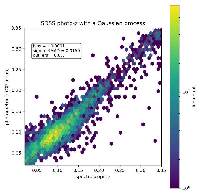
The standard photo-z metrics:
bias        = +0.0001
sigma_NMAD  = 0.0150
outlier frac= 0.025%
| The bias is essentially zero, the normalized scatter is 0.015, and almost nothing falls outside the catastrophic-outlier line at $ | \Delta z | /(1+z) > 0.15$. For bright low-redshift SDSS galaxies these are good numbers, in line with what dedicated photo-z codes report on the same regime. |
The error bars are the point
A tight scatter plot is not enough. The reason to use a GP is the variance, so the variance has to be honest. The probability integral transform checks it: for each galaxy, evaluate where the true redshift falls in the predictive Gaussian. If the error bars are right, those values are uniform on $[0, 1]$.
pit = norm.cdf((yte - mu) / sigma)
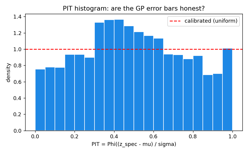
The histogram is not flat. It humps in the middle, which means the predictive intervals are slightly too wide, so the GP is a touch underconfident. That comes from the single global WhiteKernel noise term, which assigns the same scatter to every galaxy even though bright ones deserve tighter bars than faint ones. A heteroscedastic noise model would flatten it. The useful part is that the diagnostic catches this at all. The error bars are conservative rather than fragile, and now I know in which direction and why.
Scaling
The exact GP stops at a few thousand training points. Past that you move to sparse or inducing-point GPs, which keep the calibrated-uncertainty behavior while scaling to a full catalog, and if throughput matters more than honest error bars you switch to a mixture-density network instead. The GP earns its place precisely when the error bar is the product, which in cosmology it usually is.
Full code
#!/usr/bin/env python
"""Photometric redshifts with Gaussian processes, on real SDSS galaxies.

Pull ugriz photometry plus spectroscopic redshift from SDSS, train an exact GP
on colors, and predict redshift with calibrated error bars. Evaluate with the
standard photo-z metrics and a PIT histogram.
"""
import numpy as np
import matplotlib.pyplot as plt
from scipy.stats import norm
from astroquery.sdss import SDSS
from sklearn.preprocessing import StandardScaler
from sklearn.gaussian_process import GaussianProcessRegressor
from sklearn.gaussian_process.kernels import (ConstantKernel, Matern,
                                              WhiteKernel)

rng = np.random.default_rng(42)

# ---------------------------------------------------------------------------
# data: SDSS galaxies with clean photometry and a reliable spectroscopic z
# ---------------------------------------------------------------------------
QUERY = """
SELECT TOP 12000 modelMag_u, modelMag_g, modelMag_r, modelMag_i, modelMag_z, z
FROM SpecPhoto
WHERE class='GALAXY' AND zWarning=0 AND z BETWEEN 0.02 AND 0.35
AND modelMag_r BETWEEN 14 AND 19
"""
print("[photoz] querying SDSS ...")
tab = SDSS.query_sql(QUERY, timeout=300)
m = np.vstack([tab[f"modelMag_{b}"] for b in "ugriz"]).T.astype(float)
zspec = np.asarray(tab["z"], float)

# drop rows with bad magnitudes
good = np.all(np.isfinite(m), axis=1) & np.all(m > 10, axis=1) & np.all(m < 30, axis=1)
m, zspec = m[good], zspec[good]
print(f"[photoz] {len(zspec)} clean galaxies")

# features: four colors plus the r-band magnitude (a rough distance proxy)
colors = np.column_stack([m[:, 0] - m[:, 1],   # u-g
                          m[:, 1] - m[:, 2],   # g-r
                          m[:, 2] - m[:, 3],   # r-i
                          m[:, 3] - m[:, 4],   # i-z
                          m[:, 2]])            # r

# ---------------------------------------------------------------------------
# split: exact GP is O(n^3), so train on a subsample, test on the rest
# ---------------------------------------------------------------------------
idx = rng.permutation(len(zspec))
n_train = 1200
tr, te = idx[:n_train], idx[n_train:n_train + 4000]

scaler = StandardScaler().fit(colors[tr])
Xtr, Xte = scaler.transform(colors[tr]), scaler.transform(colors[te])
ytr, yte = zspec[tr], zspec[te]

kernel = (ConstantKernel(1.0) * Matern(length_scale=np.ones(Xtr.shape[1]), nu=1.5)
          + WhiteKernel(noise_level=1e-3))
gp = GaussianProcessRegressor(kernel=kernel, normalize_y=True, n_restarts_optimizer=1)
print("[photoz] fitting GP ...")
gp.fit(Xtr, ytr)
print("[photoz] learned kernel:", gp.kernel_)

mu, sigma = gp.predict(Xte, return_std=True)

# ---------------------------------------------------------------------------
# metrics
# ---------------------------------------------------------------------------
dz = (mu - yte) / (1 + yte)
bias = np.mean(dz)
nmad = 1.4826 * np.median(np.abs(dz - np.median(dz)))
outlier = np.mean(np.abs(dz) > 0.15)
print(f"[photoz] bias        = {bias:+.4f}")
print(f"[photoz] sigma_NMAD  = {nmad:.4f}")
print(f"[photoz] outlier frac= {outlier:.3%}")

# PIT: if the predictive Gaussian is calibrated, these are uniform on [0,1]
pit = norm.cdf((yte - mu) / sigma)

# ---------------------------------------------------------------------------
# figures
# ---------------------------------------------------------------------------
fig, ax = plt.subplots(figsize=(6.2, 6))
hb = ax.hexbin(yte, mu, gridsize=45, bins="log", cmap="viridis", mincnt=1)
ax.plot([0, 0.35], [0, 0.35], "r--", lw=1)
ax.set_xlim(0.02, 0.35)
ax.set_ylim(0.02, 0.35)
ax.set_aspect("equal")
ax.set_xlabel("spectroscopic z")
ax.set_ylabel("photometric z (GP mean)")
ax.set_title("SDSS photo-z with a Gaussian process")
ax.text(0.04, 0.31,
        f"bias = {bias:+.4f}\nsigma_NMAD = {nmad:.4f}\noutliers = {outlier:.1%}",
        fontsize=9, va="top",
        bbox=dict(boxstyle="round", fc="white", alpha=0.8))
fig.colorbar(hb, ax=ax, label="log count")
fig.tight_layout()
fig.savefig("uploads/2026/06/photoz-gp-scatter.png", dpi=130)
print("[photoz] saved uploads/2026/06/photoz-gp-scatter.png")

fig2, ax2 = plt.subplots(figsize=(6.5, 4))
ax2.hist(pit, bins=20, range=(0, 1), color="#1e88e5",
         edgecolor="white", density=True)
ax2.axhline(1.0, color="r", ls="--", label="calibrated (uniform)")
ax2.set_xlabel("PIT = Phi((z_spec - mu) / sigma)")
ax2.set_ylabel("density")
ax2.set_title("PIT histogram: are the GP error bars honest?")
ax2.legend()
fig2.tight_layout()
fig2.savefig("uploads/2026/06/photoz-gp-pit.png", dpi=130)
print("[photoz] saved uploads/2026/06/photoz-gp-pit.png")