I’ve been working on inference support for CyberEther, and I needed something more interesting than another image classifier to test it. So I trained a small neural network to classify asteroid spectra and connected it directly to the Gaia archive.
The result is a flowgraph that downloads real asteroid observations from a TAP service, arranges them into tensors, runs an ONNX model and plots the class probabilities live.
What is being classified?
Asteroids can be grouped by their reflectance spectra, which describe how much sunlight they reflect at different wavelengths. The Bus-DeMeo taxonomy defines around 25 classes, but I collapsed them into four broader groups:
| Group | Classes | General composition |
|---|---|---|
| C-complex | B, C, Cb, Cg, Cgh, Ch | Dark and carbon-rich |
| S-complex | S, Sa, Sq, Sr, Q, A, L | Silicate-rich |
| X-complex | X, Xe, Xc, Xk, M, E, P | Metallic or primitive |
| Other | D, T, K, V, R, O | Rare or distinct types |
The input comes from the Gaia DR3 Solar System Object catalog. Gaia provides 16 reflectance measurements for each asteroid, covering wavelengths from 374 to 990 nm. Sixteen values are not a lot, but they still capture enough of the spectral slope and absorption features to make a useful classifier.
Building the dataset
The training data comes from two public TAP services.
Gaia provides the spectra through gaiadr3.sso_reflectance_spectrum. The complete query returns 968,288 rows, representing 60,518 asteroids with up to 16 wavelength samples each. After removing incomplete spectra, 34,577 asteroids remain.
The labels come from the VizieR catalog J/A+A/665/A26, which contains Bus-DeMeo classifications collected from spectroscopic surveys. Gaia and VizieR use different identifiers, so I cross-matched them through the standard IAU minor-planet number stored in gaiadr3.sso_source.
That left me with 1,953 labeled asteroids. The class distribution is not balanced:
| Class | Samples |
|---|---|
| S-complex | 838 |
| C-complex | 533 |
| X-complex | 331 |
| Other | 251 |
This bias makes sense. Ground-based surveys are more likely to observe bright asteroids, and S-type asteroids tend to be brighter than the darker carbonaceous ones.
Training the model
I used a small scikit-learn pipeline with a StandardScaler followed by a two-layer multilayer perceptron:
pipe = Pipeline([
    ("scaler", StandardScaler()),
    ("clf", MLPClassifier(
        hidden_layer_sizes=(64, 32),
        activation="relu",
        max_iter=500,
        early_stopping=True,
    )),
])
The model architecture is 16 -> 64 -> 32 -> 4. The scaler matters because each wavelength band has a different reflectance distribution. Without normalization, the network spends too much effort dealing with scale instead of learning the shape of the spectrum.
On a held-out test set of 391 asteroids, the model reached 74.9% accuracy. That is not amazing, but it is reasonable for only 1,953 labeled examples and 16 spectral points. The original taxonomy is based on much richer spectra, so some ambiguity is unavoidable here.
I exported the complete pipeline to ONNX, including the scaler. One detail caused a bit of trouble: skl2onnx exports both the predicted label and the probability matrix by default, while CyberEther’s Infer block reads output index zero. I removed the label output from the graph so the first output became the [batch, 4] probability tensor.
The final model is only 14 KB.
Feeding live Gaia data into ONNX
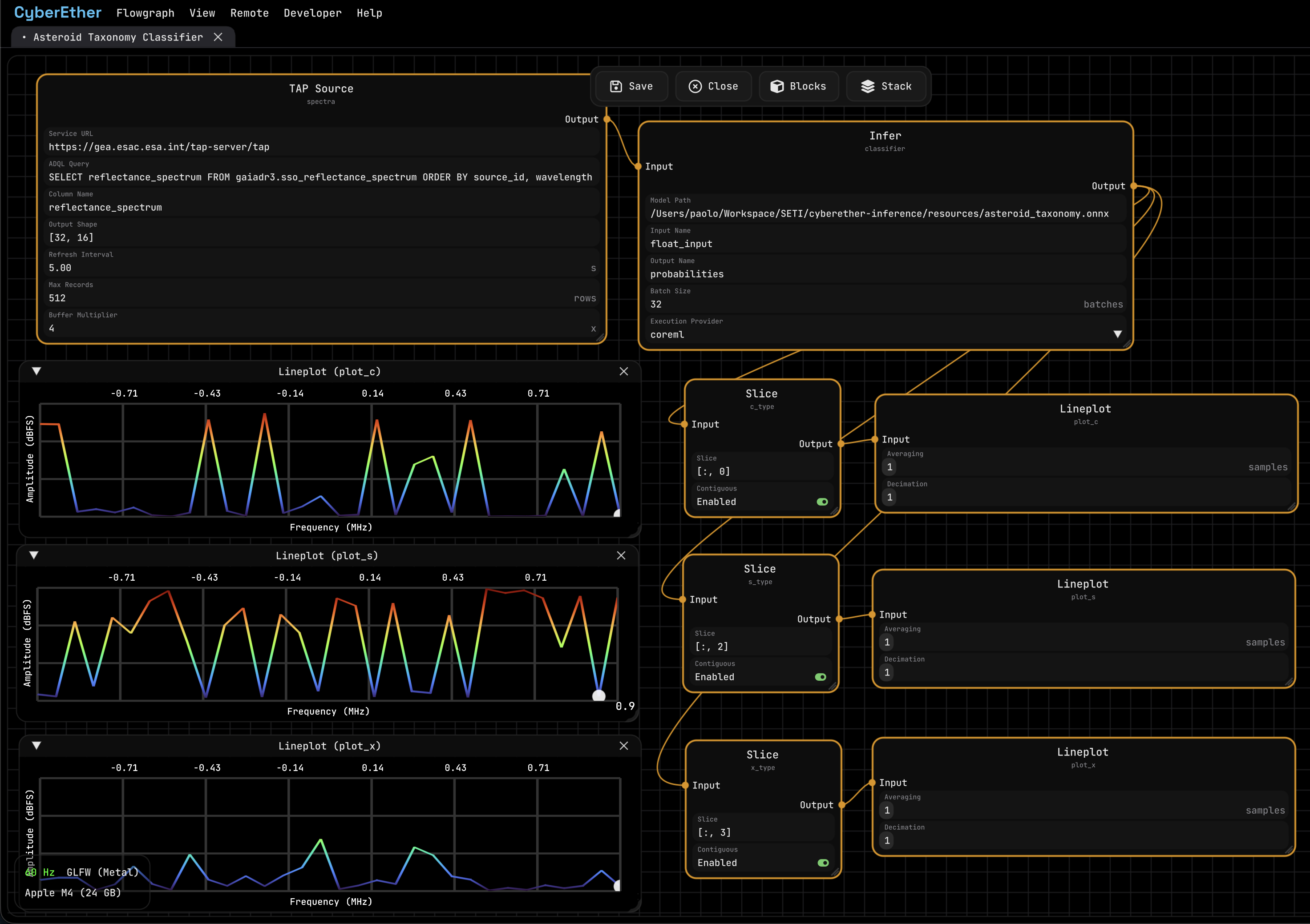
The flowgraph starts with a TAP block configured with this query:
SELECT reflectance_spectrum
FROM gaiadr3.sso_reflectance_spectrum
ORDER BY source_id, wavelength
The block requests 512 records and exposes an output tensor with shape [32, 16]. Since the query is ordered by asteroid and wavelength, every group of 16 rows is one complete spectrum. This gives the model a batch of 32 asteroids without an extra reshape step.
The Infer block runs the scaler and neural network:
StandardScaler                         [32, 16]
Dense 16 -> 64, ReLU                   [32, 64]
Dense 64 -> 32, ReLU                   [32, 32]
Dense 32 -> 4, Softmax                 [32, 4]
The four output columns follow scikit-learn’s alphabetical class order: [C, O, S, X]. I connected slices for the C, S and X probabilities to separate line plots. Each point in a plot is the probability assigned to one asteroid in the current batch.
S-type predictions are usually the clearest, with several probabilities close to one. C and X are harder to separate because reflectance alone is not always enough. Albedo data would help a lot, especially for the X-complex.
Where this can go next
The obvious limitation is the small labeled set. Around 94% of the complete Gaia spectra have no matching taxonomy label, so semi-supervised learning could be useful. Class weighting or oversampling would also reduce the S-complex bias.
Another useful improvement would be joining WISE albedo measurements into the flowgraph. That should help distinguish X-type asteroids that look similar in visible reflectance but have different physical compositions.
For now, though, I have a 14 KB model reading real astronomy data from the internet and classifying it inside a live CyberEther flowgraph. That was exactly the kind of inference test I wanted.