A single antenna sees the whole sky at once. Put several antennas together and you can make the array look in one direction, and with a bit more work you can synthesize an aperture far larger than any single dish you could build. Both tricks come from one fact: a wave arriving from an angle reaches each element at a slightly different time, which is a phase. This post builds beamforming and then aperture synthesis out of that single phasor.
One phasor, many elements
Take a uniform linear array of elements spaced by $d$. A plane wave from angle $\theta$ travels an extra distance $k\,d\sin\theta$ to reach element $k$, which is an extra phase
\[\phi_k = \frac{2\pi}{\lambda} k\,d\sin\theta\]The signal at element $k$ is the reference signal times $e^{i\phi_k}$. To listen toward a chosen direction $\theta_0$, weight each element by the conjugate of the phase it would see from $\theta_0$ and sum:
\[y(\theta_0) = \sum_k e^{-i\phi_k(\theta_0)}\, x_k\]When the array is hit by a wave from $\theta_0$, every term lines up in phase and adds coherently. From any other direction the terms have different phases and partly cancel. That is the whole mechanism.
Beamforming in code
def array_factor(n, d_over_lambda, theta, theta0):
    k = np.arange(n)[:, None]
    steer = np.exp(1j * 2 * np.pi * d_over_lambda * k * np.sin(theta0))
    resp = np.exp(1j * 2 * np.pi * d_over_lambda * k * np.sin(theta))
    return (steer.conj() * resp).sum(axis=0) / n
For a 16-element array steered to +20 degrees, the response has a narrow main lobe at the steer direction and a set of weaker side lobes everywhere else.
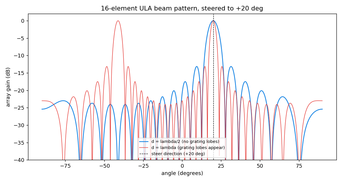
The blue curve uses half-wavelength spacing and behaves well. The red curve uses full-wavelength spacing and grows a second peak as tall as the main one, near -41 degrees. That is a grating lobe, and it is the spatial version of aliasing. The array can no longer tell +20 degrees from that mirror direction. The fix is the half-wavelength rule: keep $d \le \lambda/2$ and there is only one main lobe.
From beams to images
A correlation interferometer does not steer one beam. It correlates pairs of antennas, and each pair measures a single Fourier component of the sky brightness. The spatial frequency it samples is set by the baseline vector between the two antennas, projected onto the sky. This is the van Cittert-Zernike theorem:
\[V(u, v) = \int I(l, m)\, e^{-2\pi i (ul + vm)}\, dl\, dm\]So each baseline gives one point in the $uv$-plane. The trick that makes the whole thing work is that the Earth rotates. As the source moves across the sky, the projected baselines sweep through the $uv$-plane and fill in coverage that no fixed array could reach in a single instant.
u = (np.sin(H) * Bx + np.cos(H) * By)
v = (-np.sin(dec) * np.cos(H) * Bx
     + np.sin(dec) * np.sin(H) * By
     + np.cos(dec) * Bz)
I placed twelve antennas in a rough Y, took all 66 baselines, and tracked them across 120 degrees of hour angle, about eight hours on the sky. With the Hermitian symmetry of a real sky added in, that is about 32,000 samples in the $uv$-plane. Grid those visibilities, take an inverse FFT, and you get the dirty image: the true sky convolved with the array’s response.
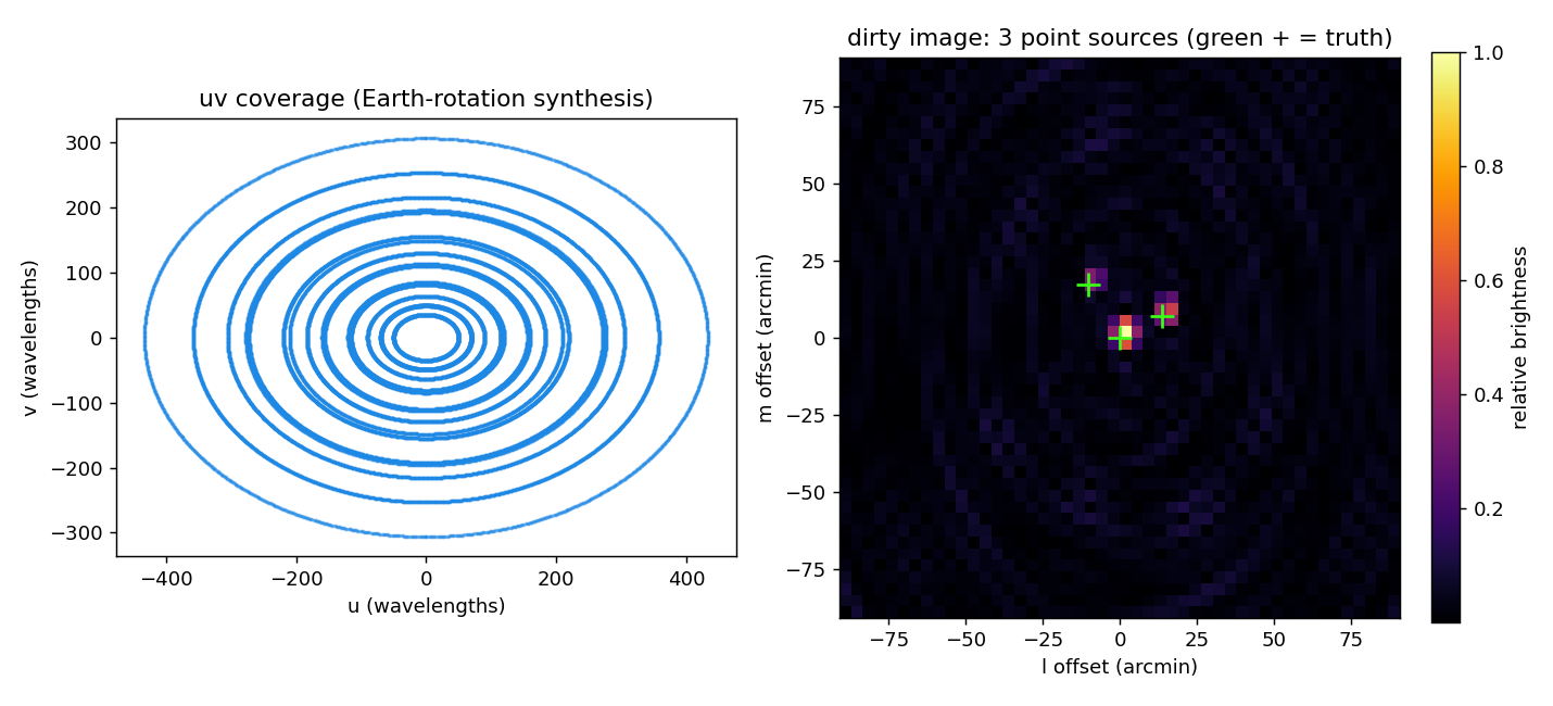
The three point sources land where they were put, each wrapped in the side-lobe pattern of the synthesized beam. Cleaning those side lobes out is what algorithms like CLEAN do, but the sources are already obvious in the raw inversion.
Why this matters for the lab
Beamforming is the bridge from the SDR hobby work to real instrument design. The same phasor that steers a phased array is the one that fills the $uv$-plane in a synthesis array, and it scales all the way up to VLBI, where the baselines span continents. For a lab built on machine learning, robotics and space, this is the signal-processing foundation the instruments sit on. You cannot reason about what a model should do with array data until you understand how the array turns the sky into numbers.
Full code
#!/usr/bin/env python
"""Beamforming and aperture synthesis from a phasor.

Part 1: steer a uniform linear array and show the beam pattern, including the
grating lobes that appear once element spacing exceeds lambda/2.

Part 2: a correlation interferometer. Earth rotation sweeps the baselines
through the uv-plane; an inverse FFT of the sampled visibilities gives the
dirty image of a small sky model.
"""
import numpy as np
import matplotlib.pyplot as plt

# ---------------------------------------------------------------------------
# Part 1: beamforming on a uniform linear array
# ---------------------------------------------------------------------------
def array_factor(n, d_over_lambda, theta, theta0):
    """Complex array response of an n-element ULA steered to theta0."""
    k = np.arange(n)[:, None]
    # steering vector a(theta0); conventional beamformer weights w = a(theta0)
    steer = np.exp(1j * 2 * np.pi * d_over_lambda * k * np.sin(theta0))
    resp = np.exp(1j * 2 * np.pi * d_over_lambda * k * np.sin(theta))
    # output w^H a(theta) peaks where theta == theta0
    return (steer.conj() * resp).sum(axis=0) / n

N = 16
thetas = np.linspace(-np.pi / 2, np.pi / 2, 2000)
theta0 = np.deg2rad(20)        # steer the main lobe to +20 degrees

af_half = np.abs(array_factor(N, 0.5, thetas, theta0))
af_full = np.abs(array_factor(N, 1.0, thetas, theta0))

def to_db(x):
    return 20 * np.log10(np.clip(x, 1e-4, None))

fig, ax = plt.subplots(figsize=(9, 4.8))
ax.plot(np.rad2deg(thetas), to_db(af_half), color="#1e88e5",
        label="d = lambda/2 (no grating lobes)")
ax.plot(np.rad2deg(thetas), to_db(af_full), color="#e53935", lw=0.9,
        label="d = lambda (grating lobes appear)")
ax.axvline(20, color="k", ls="--", lw=0.8, label="steer direction (+20 deg)")
ax.set_ylim(-40, 2)
ax.set_xlabel("angle (degrees)")
ax.set_ylabel("array gain (dB)")
ax.set_title(f"{N}-element ULA beam pattern, steered to +20 deg")
ax.legend(loc="lower center", fontsize=8)
fig.tight_layout()
fig.savefig("uploads/2026/06/beamforming-beam-pattern.png", dpi=130)
print("[fig1] saved uploads/2026/06/beamforming-beam-pattern.png")

# locate the main-lobe peak and first grating lobe of the d=lambda case
peak_deg = np.rad2deg(thetas[np.argmax(af_full)])
print(f"[fig1] d=lambda main response near {peak_deg:.1f} deg "
      f"(grating lobe mirrors the +20 deg steer)")

# ---------------------------------------------------------------------------
# Part 2: aperture synthesis by Earth rotation
# ---------------------------------------------------------------------------
rng = np.random.default_rng(20260611)

# a small 2D array layout (positions in wavelengths), vaguely Y-shaped
arms = []
for ang in [90, 210, 330]:
    a = np.deg2rad(ang)
    for r in [40, 90, 160, 250]:
        arms.append([r * np.cos(a), r * np.sin(a)])
ant = np.array(arms)                       # (Nant, 2) east, north in wavelengths
Nant = len(ant)

# baselines (Bx = east, By = north, Bz ~ 0 for a coplanar east-west array)
pairs = [(i, j) for i in range(Nant) for j in range(i + 1, Nant)]
B = np.array([ant[j] - ant[i] for i, j in pairs])     # (Nbl, 2)
Bx, By = B[:, 0], B[:, 1]
Bz = np.zeros_like(Bx)

dec = np.deg2rad(45)                        # source declination
H = np.deg2rad(np.linspace(-60, 60, 240))  # hour-angle track

# standard uvw transform, sampled over the hour-angle track
u = (np.sin(H)[:, None] * Bx + np.cos(H)[:, None] * By).ravel()
v = ((-np.sin(dec) * np.cos(H))[:, None] * Bx
     + (np.sin(dec) * np.sin(H))[:, None] * By
     + np.cos(dec) * Bz).ravel()
# Hermitian symmetry: every baseline also gives its conjugate
u = np.concatenate([u, -u])
v = np.concatenate([v, -v])

# sky model: three point sources at (l, m) offsets in radians
sources = [(0.0, 0.0, 1.0),
           (4e-3, 2e-3, 0.6),
           (-3e-3, 5e-3, 0.4)]
vis = np.zeros(u.shape, dtype=complex)
for l, m, flux in sources:
    vis += flux * np.exp(-2j * np.pi * (u * l + v * m))

# grid the visibilities and invert
npix = 256
uvmax = max(np.abs(u).max(), np.abs(v).max()) * 1.05
grid = np.zeros((npix, npix), dtype=complex)
count = np.zeros((npix, npix))
ui = ((u / uvmax + 1) / 2 * (npix - 1)).astype(int)
vi = ((v / uvmax + 1) / 2 * (npix - 1)).astype(int)
for a, b, val in zip(vi, ui, vis):
    grid[a, b] += val
    count[a, b] += 1
mask = count > 0
grid[mask] /= count[mask]

dirty = np.fft.fftshift(np.abs(np.fft.ifft2(np.fft.ifftshift(grid))))
dirty /= dirty.max()

# image pixel scale: dl = 1 / (npix * uv_cell), uv_cell = 2*uvmax/npix
dl = 1.0 / (npix * (2 * uvmax / npix))         # radians per pixel
arcmin = np.rad2deg(dl) * 60.0
# crop to the central window where the sources live
half = 24
c = npix // 2
crop = dirty[c - half:c + half, c - half:c + half]
ext = half * arcmin                            # arcmin from center

print(f"[fig2] {len(pairs)} baselines x {len(H)} samples "
      f"= {len(pairs) * len(H)} uv points (x2 with conjugates)")
print(f"[fig2] pixel scale {arcmin:.2f} arcmin, crop +/- {ext:.0f} arcmin")

fig2, ax2 = plt.subplots(1, 2, figsize=(11, 5))
ax2[0].scatter(u, v, s=1, color="#1e88e5", alpha=0.4)
ax2[0].set_aspect("equal")
ax2[0].set_title("uv coverage (Earth-rotation synthesis)")
ax2[0].set_xlabel("u (wavelengths)")
ax2[0].set_ylabel("v (wavelengths)")

im = ax2[1].imshow(crop, origin="lower", cmap="inferno",
                   extent=[-ext, ext, -ext, ext])
# mark the true source positions
for l, m, flux in sources:
    ax2[1].plot(np.rad2deg(l) * 60, np.rad2deg(m) * 60, "+",
                color="#39ff14", ms=12, mew=1.5)
ax2[1].set_title("dirty image: 3 point sources (green + = truth)")
ax2[1].set_xlabel("l offset (arcmin)")
ax2[1].set_ylabel("m offset (arcmin)")
fig2.colorbar(im, ax=ax2[1], fraction=0.046, label="relative brightness")
fig2.tight_layout()
fig2.savefig("uploads/2026/06/beamforming-uv-synthesis.png", dpi=130)
print("[fig2] saved uploads/2026/06/beamforming-uv-synthesis.png")